Two Sample Procedures
twosamp.RmdTwo-sample procedures are the basis for much research in the social and behavioral sciences. Indeed, the classic experimental setup is to establish control and treatment conditions, then randomize study participants to those conditions. The control condition is often a placebo or “traditional” intervention, and the experimental condition is a new intervention that was developed to achieve improvement, as measured by the outcome or response variable. This experimental arrangement will often lead to directional research hypotheses (e.g., those in the experimental condition will outperform those in the control condition), though two sample procedures can be used for non-directional hypotheses as well. They can also be used for observational studies for which the question of interest is whether there is a difference in a measure of units in two existing conditions (non-directional) or whether units in one condition are higher (or lower) on a measure than units in the other condition (directional).
The Fisher-Pitman procedure
As with the one-sample situation, we can use the expected outcomes under both randomization and a null hypothesis of no effect (or no difference) as motivation for a procedure to test the null hypothesis. Here is an example that we will use to build such a procedure.
Some reading experts promote Some reading experts promote direct instruction of prosodic elements (e.g., pauses, voice fluctuation) as a way to increase reading accuracy. One reading researcher conducted an experiment to compare training with repeated reading to direct prosodic instruction. The response variable was the number of errors made when reading an unfamiliar passage.
Here are the scores obtained in the study. Scores are the numbers of errors made by each study participant.
The research hypothesis is that students in the prosodic reading condition will make fewer errors than those in the repeated reading condition. If we assume that the effect is uniform across the range of readers, this means that the effect of prosodic reading will be to “shift” the distribution of reading errors in a downward direction. We can measure this shift by comparing the medians or means. This leads to either of the following hypotheses.
\(H_0: \theta_p = \theta_r\)
\(H_a: \theta_p < \theta_r\)
Alternatively, focusing on the mean rather than the median, we have these.
\(H_0: \mu_p = \mu_r\)
\(H_a: \mu_p < \mu_r\)
If the null hypothesis is true, the only reason that the particular set of scores that we observe in the prosodic instruction condition (2, 13, 11, and 15) are in that condition is because of which individuals were assigned to that condition. The score of 13, for example, is only in the prosodic instruction condition because the person who had 13 errors happened to be assigned to that condition. If that person had been assigned to the repeated reading condition, we would have observed the score of 13 in that condition. If the null hypothesis is not true, this is not the case. If prosodic reading has the effect of lowering the number of reading errors, the score of 13 may be in the prosodic reading condition because that reader made fewer errors than if he or she had not had prosodic reading instruction.
Consider a total sample size of \(n\), with \(n_p\) readers in the prosodic condition and \(n_r\) readers in the repeated reading condition, so that the total sample size is the sum of the sample size in each condition.
\(n = n_p + n_r\)
Under a true null hypothesis, each of the \(n\) choose \(n_p\) combinations of groupings that we can create from these \(n\) scores are equally likely. If the alternative hypothesis is true, we expect the smaller scores in the prosodic instruction condition. A simple statistic that we can use to measure the effectiveness of prosodic instruction is the sum of the scores in that condition. Note that if the null hypothesis is true, the set of scores in this experiment will be what we observe, and the sum of these scores will be a constant, regardless of who is assigned to each condition. Thus, observing a sum in the prosodic condition that is at or near the smallest that can be observed for that condition would have a low probability under the null hypothesis and a higher probability under the alternative hypothesis. This would provide evidence that the null hypothesis may not be true.
We can create the distribution of our test statistic (the sum of scores in the prosodic condition), under a true null hypothesis, by creating all possible combinations of our scores for sample sizes \(n_p\) and \(n_r\).
scores <- c(prosodic, repeated)
exact_twosamp_dist(scores, 4)
#>        T.val        prob     prob.up   prob.down
#>   [1,]    40 0.007936508 0.007936508 1.000000000
#>   [2,]    41 0.007936508 0.015873016 0.992063492
#>   [3,]    42 0.007936508 0.023809524 0.984126984
#>   [4,]    43 0.007936508 0.031746032 0.976190476
#>   [5,]    44 0.007936508 0.039682540 0.968253968
#>   [6,]    44 0.007936508 0.047619048 0.960317460
#>   [7,]    44 0.007936508 0.055555556 0.952380952
#>   [8,]    45 0.007936508 0.063492063 0.944444444
#>   [9,]    45 0.007936508 0.071428571 0.936507937
#>  [10,]    46 0.007936508 0.079365079 0.928571429
#>  [11,]    46 0.007936508 0.087301587 0.920634921
#>  [12,]    46 0.007936508 0.095238095 0.912698413
#>  [13,]    47 0.007936508 0.103174603 0.904761905
#>  [14,]    47 0.007936508 0.111111111 0.896825397
#>  [15,]    47 0.007936508 0.119047619 0.888888889
#>  [16,]    48 0.007936508 0.126984127 0.880952381
#>  [17,]    48 0.007936508 0.134920635 0.873015873
#>  [18,]    48 0.007936508 0.142857143 0.865079365
#>  [19,]    48 0.007936508 0.150793651 0.857142857
#>  [20,]    49 0.007936508 0.158730159 0.849206349
#>  [21,]    49 0.007936508 0.166666667 0.841269841
#>  [22,]    50 0.007936508 0.174603175 0.833333333
#>  [23,]    50 0.007936508 0.182539683 0.825396825
#>  [24,]    50 0.007936508 0.190476190 0.817460317
#>  [25,]    51 0.007936508 0.198412698 0.809523810
#>  [26,]    51 0.007936508 0.206349206 0.801587302
#>  [27,]    51 0.007936508 0.214285714 0.793650794
#>  [28,]    52 0.007936508 0.222222222 0.785714286
#>  [29,]    52 0.007936508 0.230158730 0.777777778
#>  [30,]    53 0.007936508 0.238095238 0.769841270
#>  [31,]    53 0.007936508 0.246031746 0.761904762
#>  [32,]    53 0.007936508 0.253968254 0.753968254
#>  [33,]    54 0.007936508 0.261904762 0.746031746
#>  [34,]    54 0.007936508 0.269841270 0.738095238
#>  [35,]    54 0.007936508 0.277777778 0.730158730
#>  [36,]    55 0.007936508 0.285714286 0.722222222
#>  [37,]    55 0.007936508 0.293650794 0.714285714
#>  [38,]    55 0.007936508 0.301587302 0.706349206
#>  [39,]    56 0.007936508 0.309523810 0.698412698
#>  [40,]    56 0.007936508 0.317460317 0.690476190
#>  [41,]    56 0.007936508 0.325396825 0.682539683
#>  [42,]    57 0.007936508 0.333333333 0.674603175
#>  [43,]    57 0.007936508 0.341269841 0.666666667
#>  [44,]    57 0.007936508 0.349206349 0.658730159
#>  [45,]    57 0.007936508 0.357142857 0.650793651
#>  [46,]    58 0.007936508 0.365079365 0.642857143
#>  [47,]    58 0.007936508 0.373015873 0.634920635
#>  [48,]    58 0.007936508 0.380952381 0.626984127
#>  [49,]    58 0.007936508 0.388888889 0.619047619
#>  [50,]    59 0.007936508 0.396825397 0.611111111
#>  [51,]    59 0.007936508 0.404761905 0.603174603
#>  [52,]    59 0.007936508 0.412698413 0.595238095
#>  [53,]    59 0.007936508 0.420634921 0.587301587
#>  [54,]    59 0.007936508 0.428571429 0.579365079
#>  [55,]    60 0.007936508 0.436507937 0.571428571
#>  [56,]    60 0.007936508 0.444444444 0.563492063
#>  [57,]    60 0.007936508 0.452380952 0.555555556
#>  [58,]    60 0.007936508 0.460317460 0.547619048
#>  [59,]    61 0.007936508 0.468253968 0.539682540
#>  [60,]    61 0.007936508 0.476190476 0.531746032
#>  [61,]    61 0.007936508 0.484126984 0.523809524
#>  [62,]    61 0.007936508 0.492063492 0.515873016
#>  [63,]    61 0.007936508 0.500000000 0.507936508
#>  [64,]    62 0.007936508 0.507936508 0.500000000
#>  [65,]    62 0.007936508 0.515873016 0.492063492
#>  [66,]    62 0.007936508 0.523809524 0.484126984
#>  [67,]    62 0.007936508 0.531746032 0.476190476
#>  [68,]    62 0.007936508 0.539682540 0.468253968
#>  [69,]    62 0.007936508 0.547619048 0.460317460
#>  [70,]    63 0.007936508 0.555555556 0.452380952
#>  [71,]    63 0.007936508 0.563492063 0.444444444
#>  [72,]    63 0.007936508 0.571428571 0.436507937
#>  [73,]    63 0.007936508 0.579365079 0.428571429
#>  [74,]    63 0.007936508 0.587301587 0.420634921
#>  [75,]    64 0.007936508 0.595238095 0.412698413
#>  [76,]    64 0.007936508 0.603174603 0.404761905
#>  [77,]    64 0.007936508 0.611111111 0.396825397
#>  [78,]    64 0.007936508 0.619047619 0.388888889
#>  [79,]    65 0.007936508 0.626984127 0.380952381
#>  [80,]    65 0.007936508 0.634920635 0.373015873
#>  [81,]    65 0.007936508 0.642857143 0.365079365
#>  [82,]    65 0.007936508 0.650793651 0.357142857
#>  [83,]    66 0.007936508 0.658730159 0.349206349
#>  [84,]    66 0.007936508 0.666666667 0.341269841
#>  [85,]    66 0.007936508 0.674603175 0.333333333
#>  [86,]    66 0.007936508 0.682539683 0.325396825
#>  [87,]    67 0.007936508 0.690476190 0.317460317
#>  [88,]    67 0.007936508 0.698412698 0.309523810
#>  [89,]    67 0.007936508 0.706349206 0.301587302
#>  [90,]    68 0.007936508 0.714285714 0.293650794
#>  [91,]    68 0.007936508 0.722222222 0.285714286
#>  [92,]    68 0.007936508 0.730158730 0.277777778
#>  [93,]    69 0.007936508 0.738095238 0.269841270
#>  [94,]    69 0.007936508 0.746031746 0.261904762
#>  [95,]    70 0.007936508 0.753968254 0.253968254
#>  [96,]    70 0.007936508 0.761904762 0.246031746
#>  [97,]    70 0.007936508 0.769841270 0.238095238
#>  [98,]    70 0.007936508 0.777777778 0.230158730
#>  [99,]    71 0.007936508 0.785714286 0.222222222
#> [100,]    71 0.007936508 0.793650794 0.214285714
#> [101,]    72 0.007936508 0.801587302 0.206349206
#> [102,]    72 0.007936508 0.809523810 0.198412698
#> [103,]    72 0.007936508 0.817460317 0.190476190
#> [104,]    73 0.007936508 0.825396825 0.182539683
#> [105,]    73 0.007936508 0.833333333 0.174603175
#> [106,]    73 0.007936508 0.841269841 0.166666667
#> [107,]    74 0.007936508 0.849206349 0.158730159
#> [108,]    74 0.007936508 0.857142857 0.150793651
#> [109,]    74 0.007936508 0.865079365 0.142857143
#> [110,]    74 0.007936508 0.873015873 0.134920635
#> [111,]    75 0.007936508 0.880952381 0.126984127
#> [112,]    75 0.007936508 0.888888889 0.119047619
#> [113,]    76 0.007936508 0.896825397 0.111111111
#> [114,]    76 0.007936508 0.904761905 0.103174603
#> [115,]    76 0.007936508 0.912698413 0.095238095
#> [116,]    77 0.007936508 0.920634921 0.087301587
#> [117,]    77 0.007936508 0.928571429 0.079365079
#> [118,]    77 0.007936508 0.936507937 0.071428571
#> [119,]    78 0.007936508 0.944444444 0.063492063
#> [120,]    78 0.007936508 0.952380952 0.055555556
#> [121,]    79 0.007936508 0.960317460 0.047619048
#> [122,]    79 0.007936508 0.968253968 0.039682540
#> [123,]    80 0.007936508 0.976190476 0.031746032
#> [124,]    80 0.007936508 0.984126984 0.023809524
#> [125,]    81 0.007936508 0.992063492 0.015873016
#> [126,]    83 0.007936508 1.000000000 0.007936508
The above function, exact_twosamp_dist, uses the total list of scores as the first argument and the sample size of the first sample as the second argument. Traditionally, in order to keep the test statistic distribution as small as possible, we create the distribution for the sum of scores in the smallest sample. This can be achieved with this function by putting the scores from the smallest sample first in the list of scores.
Here is our observed test statistic.
The probability of observing 41 or smaller, which is just the sum of the probabilities of observing 40 or 41, is 0.016 if the null hypothesis is true. For any tolerance for Type I errors that we have set above this value, we will reject the null hypothesis and conclude that prosodic reading has the effect of decreasing the number of errors.
Conditions for valid inference
The Fisher-Pitman randomization test for two samples is a direct competitor to the parametric t test for testing a hypothesis about the mean of two population distributions. As such, it has similar, but weaker, conditions for valid inference.
- Observations within each sample are independent of one another
- The two samples are independent of one another
- Population distributions have the same shape
The first two of these are identical to the conditions necessary for valid inference about population means when using the t test. The third condition is somewhat different. For the t test, not only do populations need to have the same shape, they must also be normally distributed. This strict condition can be relaxed when we have large sample sizes. Due to the Central Limit Theorem, the sampling distribution of the differences in means will approach that of a normal distribution as the sample size increases. The problem with reliance on this Theorem is that (a) the sample size may need to be prohibitively large in order yield a sampling distirbutin that is close enough to the normal distribution to assure us that we are observing reasonable estimates of our p values, and (b) we may be using a less efficient method of inference than other available methods.
As you read this, it is likely obvious to you that this third condition might be the most difficult of these three conditions to verify, even though it is substantially less restrictive than the normality condition. As I stated above, we can reasonably assume that our two distributions have the same shape when the effect of our treatment is uniform across the range of participant values on the response measure, so as to be responsible for a distribution “shift” in the positive or negative direction. It is this condition that enables us to test hypotheses about either the median or mean, and is also the condition that assures us that the difference in our medians will be the same as the difference in our means. This is why it does not matter which hypothesis we employ. Although a hypothesis about the means demonstrates that the randomization test is a competitor to the t test, it actually makes more sense to create hypotheses about the medians. That is because the population median is a reasonable indicator of distribution center, even when the distribution is skewed. Comparing two identically shaped skewed distributions with different medians can be accomplished with sample medians.
By now you may well be asking an obvious question: What if the effect of the treatment is not uniform? In our example, what if readers at differing levels of reading ability are influenced differently by prosodic instruction? This question can be extended to other examples and other domains. What if a particular drug has differing effects depending on the severity of the condition being treated through drug therapy? What if the magnitude of the positive effect of participation in a peer learning group is, at least in part, a function of the social characteristics of the individuals in the group? These questions all entertain the notion that there may be a moderating influence for the treatment. We can address moderator variables by including them in our study, but this requires both knowledge of the existence of such variables and subsequent measurement, which may be costly or difficult.
There is an available solution to this issue when we use a randomization test rather than relying on a mathematical model for our scores. That is to change the hypothesis of interest. Here are the hypotheses that we could use for our prosodic instruction example.
\(H_0: P(Y_p < Y_r) = 1/2\)
\(H_a: P(Y_p < Y_r) > 1/2\)
The null hypothesis tells us that if we select two scores at random, one from the treatment condition and the other from the control condition, there is a 50% chance that the score in the treatment condition will be less than that in the control condition. By contrast, the alternative hypothesis states that when we make such random draws, there is a greater than 50% chance that the score in the treatment condition will be less than that in the control condition. In research terms, this means that the treatment has the effect of reducing the number of reading errors. That is, in fact, exactly what we are interested in accomplishing. If we use such hypotheses, we only need to assume independence of observations within our conditions and independence of conditions from one another. Such conditions are easy to achieve and verify.
Using ranks
Wilcoxon suggested using the Fisher-Pitman randomization method, but doing so with ranks. We know from our experience with a single sample that not only can ranking address measurement issues (e.g., skepticism about the interval nature of scores when related to the underlying construct of interest), but it can also increase power when the tails of the distribution are heavier than what we would expect with a normal distribution. Application of this suggestion is simple: rank across all scores and then apply the method.
r.scores <- rank(scores)
exact_twosamp_dist(r.scores, 4, duplicate = FALSE)
#>       T.unique        prob     prob.up   prob.down
#>  [1,]       10 0.007936508 0.007936508 1.000000000
#>  [2,]       11 0.007936508 0.015873016 0.992063492
#>  [3,]       12 0.015873016 0.031746032 0.984126984
#>  [4,]       13 0.023809524 0.055555556 0.968253968
#>  [5,]       14 0.039682540 0.095238095 0.944444444
#>  [6,]       15 0.047619048 0.142857143 0.904761905
#>  [7,]       16 0.063492063 0.206349206 0.857142857
#>  [8,]       17 0.071428571 0.277777778 0.793650794
#>  [9,]       18 0.087301587 0.365079365 0.722222222
#> [10,]       19 0.087301587 0.452380952 0.634920635
#> [11,]       20 0.095238095 0.547619048 0.547619048
#> [12,]       21 0.087301587 0.634920635 0.452380952
#> [13,]       22 0.087301587 0.722222222 0.365079365
#> [14,]       23 0.071428571 0.793650794 0.277777778
#> [15,]       24 0.063492063 0.857142857 0.206349206
#> [16,]       25 0.047619048 0.904761905 0.142857143
#> [17,]       26 0.039682540 0.944444444 0.095238095
#> [18,]       27 0.023809524 0.968253968 0.055555556
#> [19,]       28 0.015873016 0.984126984 0.031746032
#> [20,]       29 0.007936508 0.992063492 0.015873016
#> [21,]       30 0.007936508 1.000000000 0.007936508
The sum of the ranks can range from 10 to 30. Here is the sum of the ranks for our smallest sample.
In this case, the p value is the same as what we obtained when using the original scores: 0.016. This is not always the case. If it was, using ranks would always have a relative efficiency of 1!
In addition to power concerns, an advantage of using ranks is that the test is available even with large sample sizes. That is because the ranks, and therefore the sum of ranks, is the same for a given sample size, regardless of the original scores. By contrast, a new distribution must be constructed every time we observe a new set of scores, and such distributions can become overwhelmingly large and take a substantial amount of time (even years!) to compute. Perhaps computers of the future (quantum computing?) can reduce this time to something more manageable, but at the time of this writing, large sample sizes still result in time constraints that will test both patience and human longevity.
The fact that the sum of ranks is the same (and easily calculated) for a given sample size is an especially desirable property. Here is the formula for the sum of ranks for n scores.
\(n(n + 1)/2\)
If we have two conditions, rank the scores across conditions, then calculate the sum of observed ranks in the smallest condition, we can easily calculate the sum of observed ranks in the second condition.
\([n(n + 1)/2] - \sum r_{i,1}\)
In this formula, we are summing the ranks across the i individuals in the first condition.
The fact that we can easily obtain the sum of the ranks for both conditions leads to clever algorithms for calculating the probability of sums of ranks without needing to actually compute every possible combination of scores. I am not going to present such algorithms here. I will let it suffice to give the practical result: We can conduct an exact two-sample Wilcoxon test even when we have large sample sizes. The same is not true (at least not in my lifetime) for the Fisher-Pitman randomization test with original scores.
A function for the Wilcoxon test is included in Base R. It is the same function that we used for the one-sample test, but this time we will include an additional argument (an additional set of scores) that will inform the function that we have two samples.
wilcox.test(prosodic, repeated, alternative = "less", exact = TRUE)
#>
#>  Wilcoxon rank sum test
#>
#> data:  prosodic and repeated
#> W = 1, p-value = 0.01587
#> alternative hypothesis: true location shift is less than 0
Let’s see if this will be able to handle our demand for an exact test if we have samples of size 40 and 50. I’m going to use the logistic distribution to generate scores. This distribution has slightly heaving tails than a normal distribution, so we know that using ranks will provide more power than if we use the t test with original scores.
sample.1 <- rlogis(40, location = 1, scale = 1)
sample.2 <- rlogis(50, location = 0, scale = 1)
wilcox.test(sample.1, sample.2, alternative = "greater", exact = TRUE)
#>
#>  Wilcoxon rank sum test
#>
#> data:  sample.1 and sample.2
#> W = 1243, p-value = 0.0243
#> alternative hypothesis: true location shift is greater than 0
Oh happy day!
Other extensions
As we have seen, the Fisher-Pitman method and the Wilcoxon method are really the same method. One is based on application with original scores and the other is based on application with ranks. We need not stop there. Normal scores hold great promise as replacement scores. Applying methods with normal scores guarantees that the relative efficiency, relative to the parametric counterpart, such as the t test, never slips below 1 and often provides more power, such as when we have both highly leptokurtic distributions as well as platykurtic distributions.
To apply the normal score method, we select replace original scores with normal scores, conducting our replacement with the combined samples of scores. Unlike with the one-sample procedure, this time we use both negative and positive normal scores, so we can select normal scores based on dividing the normal distribution into n + 1 parts.
\(P(Z < z_i) = i/(n + 1)\)
The nplearn package can handle this for us, so let’s use our prosodic instruction example to conduct the two-sample normal scores test. Note that the normal scores are returned to us in the same order as the scores in the vector that we submit to the function, so if we order by sample prior to obtaining the normal scores, we can retain that order when creating the distribution of the sum of the smallest sample.
n.scores <- norm_scores(scores, two.sample = TRUE)
exact_twosamp_dist(n.scores, 4)
#>                T.val        prob     prob.up   prob.down
#>   [1,] -2.900920e+00 0.007936508 0.007936508 1.000000000
#>   [2,] -2.647573e+00 0.007936508 0.015873016 0.992063492
#>   [3,] -2.394226e+00 0.007936508 0.023809524 0.984126984
#>   [4,] -2.376520e+00 0.007936508 0.031746032 0.976190476
#>   [5,] -2.123173e+00 0.007936508 0.039682540 0.968253968
#>   [6,] -2.123173e+00 0.007936508 0.047619048 0.960317460
#>   [7,] -2.059299e+00 0.007936508 0.055555556 0.952380952
#>   [8,] -1.869826e+00 0.007936508 0.063492063 0.944444444
#>   [9,] -1.852119e+00 0.007936508 0.071428571 0.936507937
#>  [10,] -1.805952e+00 0.007936508 0.079365079 0.928571429
#>  [11,] -1.805952e+00 0.007936508 0.087301587 0.920634921
#>  [12,] -1.619369e+00 0.007936508 0.095238095 0.912698413
#>  [13,] -1.598772e+00 0.007936508 0.103174603 0.904761905
#>  [14,] -1.552605e+00 0.007936508 0.111111111 0.896825397
#>  [15,] -1.534899e+00 0.007936508 0.119047619 0.888888889
#>  [16,] -1.534899e+00 0.007936508 0.126984127 0.880952381
#>  [17,] -1.366022e+00 0.007936508 0.134920635 0.873015873
#>  [18,] -1.366022e+00 0.007936508 0.142857143 0.865079365
#>  [19,] -1.345425e+00 0.007936508 0.150793651 0.857142857
#>  [20,] -1.281552e+00 0.007936508 0.158730159 0.849206349
#>  [21,] -1.281552e+00 0.007936508 0.166666667 0.841269841
#>  [22,] -1.281552e+00 0.007936508 0.174603175 0.833333333
#>  [23,] -1.217678e+00 0.007936508 0.182539683 0.825396825
#>  [24,] -1.112675e+00 0.007936508 0.190476190 0.817460317
#>  [25,] -1.094968e+00 0.007936508 0.198412698 0.809523810
#>  [26,] -1.094968e+00 0.007936508 0.206349206 0.801587302
#>  [27,] -1.028204e+00 0.007936508 0.214285714 0.793650794
#>  [28,] -1.028204e+00 0.007936508 0.222222222 0.785714286
#>  [29,] -1.010498e+00 0.007936508 0.230158730 0.777777778
#>  [30,] -9.643308e-01 0.007936508 0.238095238 0.769841270
#>  [31,] -8.416212e-01 0.007936508 0.246031746 0.761904762
#>  [32,] -8.416212e-01 0.007936508 0.253968254 0.753968254
#>  [33,] -8.416212e-01 0.007936508 0.261904762 0.746031746
#>  [34,] -7.777476e-01 0.007936508 0.269841270 0.738095238
#>  [35,] -7.777476e-01 0.007936508 0.277777778 0.730158730
#>  [36,] -7.571511e-01 0.007936508 0.285714286 0.722222222
#>  [37,] -7.571511e-01 0.007936508 0.293650794 0.714285714
#>  [38,] -7.109837e-01 0.007936508 0.301587302 0.706349206
#>  [39,] -6.932774e-01 0.007936508 0.309523810 0.698412698
#>  [40,] -5.882741e-01 0.007936508 0.317460317 0.690476190
#>  [41,] -5.882741e-01 0.007936508 0.325396825 0.682539683
#>  [42,] -5.705678e-01 0.007936508 0.333333333 0.674603175
#>  [43,] -5.244005e-01 0.007936508 0.341269841 0.666666667
#>  [44,] -5.244005e-01 0.007936508 0.349206349 0.658730159
#>  [45,] -5.244005e-01 0.007936508 0.357142857 0.650793651
#>  [46,] -5.038039e-01 0.007936508 0.365079365 0.642857143
#>  [47,] -4.399303e-01 0.007936508 0.373015873 0.634920635
#>  [48,] -4.399303e-01 0.007936508 0.380952381 0.626984127
#>  [49,] -3.378173e-01 0.007936508 0.388888889 0.619047619
#>  [50,] -3.172207e-01 0.007936508 0.396825397 0.611111111
#>  [51,] -3.172207e-01 0.007936508 0.404761905 0.603174603
#>  [52,] -2.710534e-01 0.007936508 0.412698413 0.595238095
#>  [53,] -2.710534e-01 0.007936508 0.420634921 0.587301587
#>  [54,] -2.533471e-01 0.007936508 0.428571429 0.579365079
#>  [55,] -2.533471e-01 0.007936508 0.436507937 0.571428571
#>  [56,] -2.533471e-01 0.007936508 0.444444444 0.563492063
#>  [57,] -1.865832e-01 0.007936508 0.452380952 0.555555556
#>  [58,] -1.688769e-01 0.007936508 0.460317460 0.547619048
#>  [59,] -8.447018e-02 0.007936508 0.468253968 0.539682540
#>  [60,] -6.387362e-02 0.007936508 0.476190476 0.531746032
#>  [61,]  0.000000e+00 0.007936508 0.484126984 0.523809524
#>  [62,]  0.000000e+00 0.007936508 0.492063492 0.515873016
#>  [63,]  0.000000e+00 0.007936508 0.500000000 0.507936508
#>  [64,]  2.220446e-16 0.007936508 0.507936508 0.500000000
#>  [65,]  2.220446e-16 0.007936508 0.515873016 0.492063492
#>  [66,]  2.220446e-16 0.007936508 0.523809524 0.484126984
#>  [67,]  6.387362e-02 0.007936508 0.531746032 0.476190476
#>  [68,]  8.447018e-02 0.007936508 0.539682540 0.468253968
#>  [69,]  1.688769e-01 0.007936508 0.547619048 0.460317460
#>  [70,]  1.865832e-01 0.007936508 0.555555556 0.452380952
#>  [71,]  2.533471e-01 0.007936508 0.563492063 0.444444444
#>  [72,]  2.533471e-01 0.007936508 0.571428571 0.436507937
#>  [73,]  2.533471e-01 0.007936508 0.579365079 0.428571429
#>  [74,]  2.710534e-01 0.007936508 0.587301587 0.420634921
#>  [75,]  2.710534e-01 0.007936508 0.595238095 0.412698413
#>  [76,]  3.172207e-01 0.007936508 0.603174603 0.404761905
#>  [77,]  3.172207e-01 0.007936508 0.611111111 0.396825397
#>  [78,]  3.378173e-01 0.007936508 0.619047619 0.388888889
#>  [79,]  4.399303e-01 0.007936508 0.626984127 0.380952381
#>  [80,]  4.399303e-01 0.007936508 0.634920635 0.373015873
#>  [81,]  5.038039e-01 0.007936508 0.642857143 0.365079365
#>  [82,]  5.244005e-01 0.007936508 0.650793651 0.357142857
#>  [83,]  5.244005e-01 0.007936508 0.658730159 0.349206349
#>  [84,]  5.244005e-01 0.007936508 0.666666667 0.341269841
#>  [85,]  5.705678e-01 0.007936508 0.674603175 0.333333333
#>  [86,]  5.882741e-01 0.007936508 0.682539683 0.325396825
#>  [87,]  5.882741e-01 0.007936508 0.690476190 0.317460317
#>  [88,]  6.932774e-01 0.007936508 0.698412698 0.309523810
#>  [89,]  7.109837e-01 0.007936508 0.706349206 0.301587302
#>  [90,]  7.571511e-01 0.007936508 0.714285714 0.293650794
#>  [91,]  7.571511e-01 0.007936508 0.722222222 0.285714286
#>  [92,]  7.777476e-01 0.007936508 0.730158730 0.277777778
#>  [93,]  7.777476e-01 0.007936508 0.738095238 0.269841270
#>  [94,]  8.416212e-01 0.007936508 0.746031746 0.261904762
#>  [95,]  8.416212e-01 0.007936508 0.753968254 0.253968254
#>  [96,]  8.416212e-01 0.007936508 0.761904762 0.246031746
#>  [97,]  9.643308e-01 0.007936508 0.769841270 0.238095238
#>  [98,]  1.010498e+00 0.007936508 0.777777778 0.230158730
#>  [99,]  1.028204e+00 0.007936508 0.785714286 0.222222222
#> [100,]  1.028204e+00 0.007936508 0.793650794 0.214285714
#> [101,]  1.094968e+00 0.007936508 0.801587302 0.206349206
#> [102,]  1.094968e+00 0.007936508 0.809523810 0.198412698
#> [103,]  1.112675e+00 0.007936508 0.817460317 0.190476190
#> [104,]  1.217678e+00 0.007936508 0.825396825 0.182539683
#> [105,]  1.281552e+00 0.007936508 0.833333333 0.174603175
#> [106,]  1.281552e+00 0.007936508 0.841269841 0.166666667
#> [107,]  1.281552e+00 0.007936508 0.849206349 0.158730159
#> [108,]  1.345425e+00 0.007936508 0.857142857 0.150793651
#> [109,]  1.366022e+00 0.007936508 0.865079365 0.142857143
#> [110,]  1.366022e+00 0.007936508 0.873015873 0.134920635
#> [111,]  1.534899e+00 0.007936508 0.880952381 0.126984127
#> [112,]  1.534899e+00 0.007936508 0.888888889 0.119047619
#> [113,]  1.552605e+00 0.007936508 0.896825397 0.111111111
#> [114,]  1.598772e+00 0.007936508 0.904761905 0.103174603
#> [115,]  1.619369e+00 0.007936508 0.912698413 0.095238095
#> [116,]  1.805952e+00 0.007936508 0.920634921 0.087301587
#> [117,]  1.805952e+00 0.007936508 0.928571429 0.079365079
#> [118,]  1.852119e+00 0.007936508 0.936507937 0.071428571
#> [119,]  1.869826e+00 0.007936508 0.944444444 0.063492063
#> [120,]  2.059299e+00 0.007936508 0.952380952 0.055555556
#> [121,]  2.123173e+00 0.007936508 0.960317460 0.047619048
#> [122,]  2.123173e+00 0.007936508 0.968253968 0.039682540
#> [123,]  2.376520e+00 0.007936508 0.976190476 0.031746032
#> [124,]  2.394226e+00 0.007936508 0.984126984 0.023809524
#> [125,]  2.647573e+00 0.007936508 0.992063492 0.015873016
#> [126,]  2.900920e+00 0.007936508 1.000000000 0.007936508
Here is the sum in the prosodic instruction condition.
As before, we obtain p = 0.016. Looking at this distribution highlights what may be the only disadvantage of using the normal scores test. As with original scores, the distribution can become large very quickly. Until computers become even more powerful, the Wilcoxon will still be our go-to procedure for large sample sizes.
You may recall from our study of a single sample that the sign test, although it is based on the binomial distribution, can be conducted using the one-sample randomization model simply by replacing scores with values of 0 and 1, to represent the dichotomous nature of the sign test. Similarly, instead of using the hypergeometric distribution to conduct the Fisher-Irwin test, we can perform this test as a randomization test with 0 and 1 values.
Here is the method we used to analyze band performance data with a fixed number of successes at 5, in order to fill the all-state band slots.
morning.success <- 0:5
afternoon.success <- 5 - morning.success
delta.hat <- morning.success/10 - afternoon.success/10
prob <- dhyper(morning.success, 10, 10, 5)
cbind(morning.success, afternoon.success, delta.hat, prob)
#>      morning.success afternoon.success delta.hat       prob
#> [1,]               0                 5      -0.5 0.01625387
#> [2,]               1                 4      -0.3 0.13544892
#> [3,]               2                 3      -0.1 0.34829721
#> [4,]               3                 2       0.1 0.34829721
#> [5,]               4                 1       0.3 0.13544892
#> [6,]               5                 0       0.5 0.01625387
Let’s do this again using our exact two-sample distribution procedure and replacing scores with 0s and 1s. We will have 5 successes and 15 failures, so I am going to put 5 values of 1 and 15 values of 0 into the function. I’ll also indicate that the size of the first sample is 10.
exact_twosamp_dist(c(rep(1, 5), rep(0, 15)), 10, duplicate = FALSE)
#>      T.unique       prob    prob.up  prob.down
#> [1,]        0 0.01625387 0.01625387 1.00000000
#> [2,]        1 0.13544892 0.15170279 0.98374613
#> [3,]        2 0.34829721 0.50000000 0.84829721
#> [4,]        3 0.34829721 0.84829721 0.50000000
#> [5,]        4 0.13544892 0.98374613 0.15170279
#> [6,]        5 0.01625387 1.00000000 0.01625387
We get the same distribution using randomization as we do using the hypergeometric! Cool! So we can envision the Fisher-Irwin test as the Fisher-Pitman randomization test, but using 0 and 1 as replacement scores.
A confidence interval for the median difference
Consider the following difference, where \(x_1\) is a score from our first sample and \(x_2\) is a score from our second sample.
\(d = X_2 - X_1\)
We can create all possible differences between scores in our first and second samples. Here is a matrix for our prosodic instruction example.
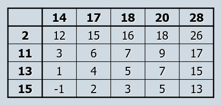
Figure 2
Under the null hypothesis, we would expect the median of these difference scores to be 0. That is, we could rewrite the null and alternative hypothesis like this.
\(H_0: \theta_d = 0\)
\(H_a: \theta_d > 0\)
Note that the direction of our alternative hypothesis depends on the direction of subtraction in the matrix. In this example, I have subtracted the errors in the prosodic instruction condition from those in the repeated reading condition, so if prosodic instruction is reducing the number of errors, then I am expecting a positive difference.
We can obtain an estimate of \(\theta_d\) by using \(\hat{\theta}_d\), the median of these differences. Note that unlike the mean, the median of the differences is not guaranted to be equal to the difference of the medians. While both of these statistics provide an estimate of the effectiveness of prosodic instruction, the median of differences will be a more generally useful estimate.
In the late 40s, at about the same time that Wilcoxon was developing his two-sample test based on ranks, two statisticians by the names of Henry Mann and Donald Whitney developed a test based on all possible differences. They defined an “inversion” with the following definition.
\(d > \theta_d\)
They then referred to the number of inversions as “U”, so their test is commonly known as the Mann-Whitney U test. If the null hypothesis is true, we should expect U to be half of the total number of differences. If the alternative hypothesis is true, and based on the way I subtracted in the above matrix, we would expect U to be a larger number. Mann and Whitney then computed probabilities for U, given the truth of the null hypothesis. Using these probabilities, we can conduct a test of the null hypothesis to determine whether we should reject it in favor of the alternative hypothesis.
It turns out that U can be written as a function of Wilcoxon’s T, the sum of the differences in the smallest group. Here’s the formula.
\(U = n_1 n_2 + \frac{n_1(n_1 + 1)}{2} - T\)
Here again is the distribution of T for our prosodic instruction example.
exact_twosamp_dist(r.scores, 4, duplicate = FALSE)
#>       T.unique        prob     prob.up   prob.down
#>  [1,]       10 0.007936508 0.007936508 1.000000000
#>  [2,]       11 0.007936508 0.015873016 0.992063492
#>  [3,]       12 0.015873016 0.031746032 0.984126984
#>  [4,]       13 0.023809524 0.055555556 0.968253968
#>  [5,]       14 0.039682540 0.095238095 0.944444444
#>  [6,]       15 0.047619048 0.142857143 0.904761905
#>  [7,]       16 0.063492063 0.206349206 0.857142857
#>  [8,]       17 0.071428571 0.277777778 0.793650794
#>  [9,]       18 0.087301587 0.365079365 0.722222222
#> [10,]       19 0.087301587 0.452380952 0.634920635
#> [11,]       20 0.095238095 0.547619048 0.547619048
#> [12,]       21 0.087301587 0.634920635 0.452380952
#> [13,]       22 0.087301587 0.722222222 0.365079365
#> [14,]       23 0.071428571 0.793650794 0.277777778
#> [15,]       24 0.063492063 0.857142857 0.206349206
#> [16,]       25 0.047619048 0.904761905 0.142857143
#> [17,]       26 0.039682540 0.944444444 0.095238095
#> [18,]       27 0.023809524 0.968253968 0.055555556
#> [19,]       28 0.015873016 0.984126984 0.031746032
#> [20,]       29 0.007936508 0.992063492 0.015873016
#> [21,]       30 0.007936508 1.000000000 0.007936508
If we conducted the test using a 5% Type I error rate, our critical value would be 12. Let’s plug that into the above equation.
\(U = (4)(5) + \frac{(4)(4+1)}{2} - 12 = 18\)
This is the critical value if we use the Mann-Whitney U. Out of the 20 median differences, we will reject the null hypothesis if we have 18, 19, or 20 inversions. We have 19, so we will reject the null hypothesis. We knew that would happen because we rejected the null hypothesis with the two-sample Wilcoxon test, and we have now seen that these tests are equivalent.
If they are equivalent, why bother presenting this second test? I’m glad you asked! With the Mann-Whitney U procedure, we could test these hypotheses.
\(H_0: \theta_d = 1\)
\(H_a: \theta_d > 1\)
All we need to do is to subtract 1 from all the values in our matrix in order to change the null hypothesis back to a median difference of 0. Look at the matrix. If we subtract 1, we will now have 18 inversions (U = 18). If we test for a median difference of 2, we just subtract 2 from all values. We now have U = 17. If we subtract 3, we now have U = 15.
But wait! We know that we will reject the null hypothesis for U = 18, 19, or 20. That means we will reject for a hypothesized median difference of 1, but we will not reject for a hypothesized median difference of 2. We also will not reject for a hypothesized median difference of 3. It doesn’t take long to figure out that 2 is a cut-off value between rejecting the null hypothesis (any median difference less than 2) or retaining the null hypothesis (any median difference of 2 or greater). A confidence interval consists of all null hypotheses that we do not reject, given our observations, so we now have a confidence interval! A 95% confidence interval for the median difference is given by this.
\(\theta_d \ge 2\)
Do we have to build this matrix every time we want a confidence interval? We do not. Check it out.
wilcox.test(repeated,
            prosodic,
            alternative = "greater",
            exact = TRUE,
            conf.int = TRUE)
#>
#>  Wilcoxon rank sum test
#>
#> data:  repeated and prosodic
#> W = 19, p-value = 0.01587
#> alternative hypothesis: true location shift is greater than 0
#> 95 percent confidence interval:
#>    2 Inf
#> sample estimates:
#> difference in location
#>                      7
Life just keeps getting better and better!