The Fisher-Irwin Test • nplearn

When we have two independent samples and a dichotomous response variable, our interest is in the probability of a joint event in which there are some number of successes in one sample and some number of successes in the other sample. Other than the sample size, there is no restriction on how many successes can occur in each sample. In some situations, however, the total number of successes is known in advance. In that case, the number of successes in our two conditions are dependent on one another. Knowing the number of successes in one condition will tell us the number in the other condition. In this vignette, we turn our attention to analyzing data when the number of successes is known prior to the start of the study.

Required packages

The packages required for this vignette are nplearn and MASS. Make certain that you have installed these packages before attempting to load the libraries.

library(nplearn)
library(MASS)

The hypergeometric distribution

In the product binomial vignette, we analyzed data obtained from two samples created by randomizing 20 band students to morning and afternoon tryouts for the all-state band. Let’s again consider this scenario, but this time suppose that these students all come from one school. The all-state band committee has indicated how many students can be accepted from each school, based on school size. For this school, only five slots can be filled by band members from the school.

Here are the (hypothetical) data.

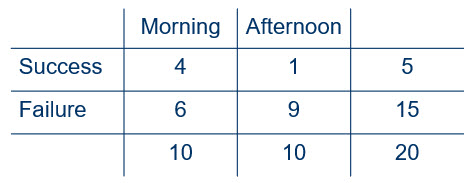
Figure 1

As in the previous example, 20 students were randomly assigned to morning and afternoon tryout conditions. The difference this time is that we know before the tryouts even begin that there will be 5 successes. Notice that with this knowledge we can fill in every margin in our table before we ever collect the data. This is clearly not a product binomial problem because the number of possible successes do not vary from 0 to 10 for each condition. The highest number of successes that can occur in a condition is 5. Further, the number of successes that can occur in the other condition is directly related to how many there are in the first condition so that the numbers of successes must sum to 5.

We can conceive of the possibilities by focusing on just one cell in this four cell crossbreak table. Let’s focus on the upper left cell (morning successes). This can range from 0 to 5 successes. Notice that whatever value we set this cell to be in that range, the entire table can be completed. We already know that we cannot calculate the probability of this table with the product binomial formula, so what do we do?

The answer is that under the null hypothesis of equal proportions of successes in both morning and afternoon conditions, the probability of a particular value of \(\hat{\delta}\) is given by the hypergeometric formula. We can use a function in R to make this calculation. For example, for our oberved data in Figure 1, here is the probability calculation.

dhyper(4, 10, 10, 5)
#> [1] 0.1354489

The entry of values is for obtaining the probability of randomly selecting 4 morning students out of 10 morning students when we also have 10 afternoon students and there will be 5 slots to fill.

Realizing that number of morning successes can only range from 0 to 5, and also knowing that the remainder of the success will be in the afternoon, we can create the entire probability distribution.

morning.success <- 0:5
afternoon.success <- 5 - morning.success
delta.hat <- morning.success/10 - afternoon.success/10
prob <- dhyper(morning.success, 10, 10, 5)
cbind(morning.success, afternoon.success, delta.hat, prob)
#>      morning.success afternoon.success delta.hat       prob
#> [1,]               0                 5      -0.5 0.01625387
#> [2,]               1                 4      -0.3 0.13544892
#> [3,]               2                 3      -0.1 0.34829721
#> [4,]               3                 2       0.1 0.34829721
#> [5,]               4                 1       0.3 0.13544892
#> [6,]               5                 0       0.5 0.01625387

Here’s a check that these probabilities sum to 1.

sum(prob)
#> [1] 1

Suppose we are looking for judging bias in either direction (i.e. favoring either the morning or afternoon). Then we need to obtain our p value we need to add up all the probabilities for absolute values of \(\hat{\delta}\) that are at least as great as our observed value of 0.3.

sum(prob[abs(delta.hat) >= 0.3])
#> [1] 0.3034056

Clearly this is insufficient evidence to make claims of judging bias. If we had set out to study whether there is bias in favor of morning sessions, we would have just looked at one side of the distribution.

sum(prob[delta.hat >= 0.3])
#> [1] 0.1517028

This still is probably not enough evidence for us to make bias accusations, even though we did find that 40% of the morning students and only 10% of the afternoon students were selected. The sample size is simply not large enough for us to claim bias, even with this estimate of time-of-day effect.

A test for median equality

When the response variable for a single sample yields quantitative data, we can use the sign test as a test of a hypothesis about the median. Similarly, the Fisher-Irwin test can be used as a test of a hypothesis about the equality of two medians.

To exemplify this method, consider an example in which an independent evaluation firm interviews employees at 12 companies and then, based on the results of the interview, gives each company an “employee satisfaction score.” Some of these companies have put an employee feedback system (EFS) in place as a means for employees to communicate concerns to management. The primary question is whether companies with such systems have higher satisfaction scores than those without such systems. We can view these companies as representing a larger population of companies, some of which have EFS and some which do not. Our interest is in whether the median satisfaction score is greater for companies with feedback systems than for companies that have not implemented such a system. Let’s input the scores for this hypothetical example.

efs <- c(8, 5, 8, 10, 9, 10, 11)
no.efs <- c(4, 7, 7, 4, 5)

Here are the null and alternative hypotheses.

\(H_0: \theta_{efs} = \theta_{no \: efs}\)

\(H_a: \theta_{efs} > \theta_{no \: efs}\)

If the null hypothesis is true, the two types of companies share the same median, so to estimate this common median we can combine all scores.

all.companies <- c(efs, no.efs)
median(all.companies)
#> [1] 7.5

Let us now look at how many companies are above the median in each of the two conditions.

sum(efs > 7.5)
#> [1] 6
sum(no.efs > 7.5)
#> [1] 0

With this information in hand, we can construct the following table.

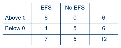
Figure 2

As with the previous Fisher-Irwin example, all margin totals are known before the interviews are conducted and the companies are scored. We know which of the the companies have EFS in place, so the two sample sizes are known. The fact that we have hypothesized a common median tells us that half of the companies will be above the median and half will be below the median, so this margin is known as well. We can think of being above the median as a “success” and being below as a “failure,” so this is the same type of situation as we had in the Fisher-Irwin example, so we can use the hypergeometric distribution.

efs.above <- 1:6
no.efs.above <- 6 - efs.above
delta.hat <- efs.above/7 - no.efs.above/5
prob <- dhyper(efs.above, 7, 5, 6)
cbind(efs.above, no.efs.above, delta.hat, prob)
#>      efs.above no.efs.above  delta.hat        prob
#> [1,]         1            5 -0.8571429 0.007575758
#> [2,]         2            4 -0.5142857 0.113636364
#> [3,]         3            3 -0.1714286 0.378787879
#> [4,]         4            2  0.1714286 0.378787879
#> [5,]         5            1  0.5142857 0.113636364
#> [6,]         6            0  0.8571429 0.007575758

This is a one-sided test, so we can see that for the observed difference in proportions of 0.86, the p value is 0.0076. We can declare that EFS makes a difference in employee satisfaction, though there is a caveat: the data are from an observational study, rather than from an experiment. Extraneous variables may be responsible for the satisfaction differences. For example, suppose that the same companies that care enough about employee opinion to solicit feedback are also the companies that care enough to implement other employee-focused initiatives, such as break facility improvements or bonus incentives. These may be responsible for the difference, rather than the EFS.

Instead of looking at the full distribution, we can use a function that is available in R.

efs.table <- matrix(c(6, 0, 1, 5),
                    nrow = 2,
                    byrow = TRUE)

fisher.test(efs.table, alternative = "greater")
#> 
#>  Fisher's Exact Test for Count Data
#> 
#> data:  efs.table
#> p-value = 0.007576
#> alternative hypothesis: true odds ratio is greater than 1
#> 95 percent confidence interval:
#>  2.4008    Inf
#> sample estimates:
#> odds ratio 
#>        Inf

We observe that the p value matches what we calculated earlier. We also notice a confidence interval for the “odds ratio,” so now would be a good time to learn about this statistic.

The odds ratio

In the previous example, the estimated proportion of EFS companies that are above the median company satisfaction score is 6/7, or 0.86. For the non-EFS companies it is 0/5, or 0. The odds of a specified outcome is the ratio of the expected frequency of that outcome to that of another outcome. In the current example, this would be the expected frequency of a company being above the median to that of being below the median. Obviously we don’t know this expected frequency. It is a population value. What we do know, however are the observed frequencies, so we can use these to estimate the population values.

The odds of an EFS company being above the median are estimated to be 6 to 1, because 6 companies are above the median and 1 is below. If we consider this as a ratio, this is 6/1, or 6. This means that there is a six times greater chance for an EFS company being above the median than below the median.

Estimating the odds for a non-EFS company gives us a peculiar result: It is 0 to 5, or 0/5, or 0. Stating that there is a “0 times greater chance” of being above the median than below the median is likely due to the small sample size. We would assume that with a larger number of companies, we would find some of them above the median satisfaction score, even if they had not implemented a feedback system.

The ratio of the odds, better known as the odds ratio is quite simply a ratio of these two odds. In the current example, we have (6/1)/(0/5). Again, we get a peculiar result due to the small sample size: 6/0. Dividing a number by 0 gives us an infinite result, which is why the odds ratio reported by the function above is listed as “inf”. Even with this peculiar result, the confidence interval for the odds ratio was calculated as 2.4 to infinity. This means we are 95% confident that for the population of companies, implementation of an EFS makes it between 2.4 times to “infinite times” more likely to result in a satisfaction score that is above the median satisfaction score of all companies.

Let’s do this again with the band data so that we can see an example without the peculiarity of having “infinite” in our results. Remember that this was a two-sided test because we were looking for judging bias in either direction.

morning.odds <- 4/6
afternoon.odds <- 1/9
odds.ratio <- morning.odds/afternoon.odds
odds.ratio
#> [1] 6

This tells us that based on our observed data, we estimate that the chance of being selected for the all-state band is 6 times greater if you are judged in the morning than if you are judged in the afternoon. This is substantial, but remember that with the small sample size, this was not enough evidence to conclude that this is judging bias. Let’s look at it with the R function.

band.table <- matrix(c(4, 1, 6, 9),
                     nrow = 2,
                     byrow = TRUE)

fisher.test(band.table)
#> 
#>  Fisher's Exact Test for Count Data
#> 
#> data:  band.table
#> p-value = 0.3034
#> alternative hypothesis: true odds ratio is not equal to 1
#> 95 percent confidence interval:
#>    0.4075889 326.8267297
#> sample estimates:
#> odds ratio 
#>   5.485861

You may notice that the estimate of the odds ratio, about 5.5, is different than the odds ratio that we obtained of 6. Why? The sample odds ratio (our simple calculation above) can be calculated regardless of the number of marginal values that are fixed. That is, it does not “know” that we specified that there are only 5 slots available for the all-state band. If the judges changed it to be 6 slots, we would still get the same estimate (6) of the odds ratio. Yet how can this be? If there are fewer slots, the odds should change! The way to deal with this is to calculate an odds ratio that is conditioned on our fixed margins. Showing how to do this “by hand” is beyond what were we are going to go, but that’s OK because the R function is doing exactly that for us. The estimate it reports is actually a better estimate than the simple one we calculated above, so we just need to focus on interpretation. The chance of success in a morning slot is about 5.5 times the chance of success in an afternoon slot.

Look at the confidence interval. It ranges from saying that the chance of success in the morning is less than half the chance of success in the afternoon all the way to the chance in the morning being 327 times the chance of success in the afternoon! This huge interval is consistent with our large p value. Clearly we could benefit from a larger sample.