The Product Binomial
ProdBinom.RmdIn this vignette we will consider the comparison of two populations on a dichotomous response variable. We analyzed a dichotomous variable for a single population with the help of the binomial distribution. Similarly, we will compare two populations on a dichotomous response with the help of the product binomial distribution.
Required packages
The packages required for this vignette are nplearn and MASS. Make certain that you have installed these packages before attempting to load the libraries.
Descriptive comparison of two populations on a dichotomous response
High school band teachers occasionally complain that judges in an all-state band competition are biased toward certain times of the day. Suppose that to examine this claim a researcher randomly divided 20 students who were trying out for all-state band into two groups, then arranged to have tryouts for members of one group in the morning and members of the other group in the afternoon. The response of interest is success or failure in being selected for the all-state band.
In this example there are two independent populations of interest: students who have a morning tryout time and students who have an afternoon tryout time. The 20 students in the study represent these two populations, with 10 students representing one population and 10 representing the other population. As always, the degree of representation depends on the method of selection, with random sampling assuring the removal of sampling bias. The fact that the students were randomized to conditions addresses extraneous variables, most important among these being the students instrument playing ability. If the study reveals a selection bias based on time of day, we can be confident, with a specified degree of probability, that it is indeed the time of day that seems to sway the judges one way or the other.
Suppose that the results of the tryouts are as shown in Figure 1.
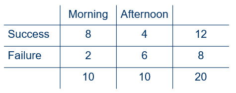
Figure 1
Here is our best estimate of the success rate for the population of students trying out for band in the morning.
\(\hat{\pi}_1 = 8/10 = 0.80\)
Here is our best estimate for the success rate for the population of students trying out for band in the afternoon.
\(\hat{\pi}_2 = 4/10 = 0.40\)
Clearly those trying out in the morning had a better rate of success. We can estimate that rate difference like this.
\(\hat{\delta} = \hat{\pi}_1 - \hat{\pi}_2 = 0.80 - 0.40 = 0.40\)
Here we are using \(\hat{\delta}\) to estimate \(\delta\). We can view \(\delta\) as the difference in population proportions, or as the difference in the probability of success between morning and afternoon tryouts.
As with any statistic, \(\hat{\delta}\) will vary. Selecting a new sample or even re-randomizing the selected sample is likely to produce different values of \(\hat{\delta}\). We would hope that the student performance in the tryout is a much larger contribution to selection than the time of day, so who happens to be in each condition when we randomize is certainly in play. We have not “equalized” the conditions by randomizing, but rather have eliminated systematic bias that would favor one condition over the other. To determine if the different success rates for the different time of days appear to be due to something other than the randomization process, we are going to need to do an analysis that will allow us to infer such a difference.
The product binomial
Consider \(n_1\) independent observations in which the probability of observing a success for each observation is \(\pi_1\). The probability of a specified number of successes is given by the binomial formula.
\(P(X_1 = x_1) = \binom{n_1}{x_1}\pi_1^{x_1}(1-\pi_1)^{(n_1-x_1)}\)
In this formula, \(x_1\) represents the number of successes observed in the \(n_1\) observations.
If we now take a second set of \(n_2\) indpendent observations in which the probability of observing a success for each observation is \(\pi_2\), the probability of observing a specified number of successes, \(x_2\) is also given by the binomial formula.
\(P(X_2 = x_2) = \binom{n_2}{x_2}\pi_2^{x_2}(1-\pi_2)^{(n_2-x_2)}\)
If it is the case that each of the \(n_1\) observations are also independent of the \(n_2\) observations, then we can find the joint probability of \(x_1\) and \(x_2\) successes by taking the product of the individual probabilities.
\(P(X_1 = x_1)*P(X_2 = x_2)\)
This is referred to the product binomial. If we vary the number of successes in order to include all possibilities (i.e., 0 to \(n_1\) and 0 to \(n_2\)), we can create the complete probability distribution based on the product binomial. Given that we can calculate \(\hat{\delta}\) for all combinations of \(x_1\) and \(x_2\), this distribution would be the probability distribution for \(\hat{\delta}\).
Here is the distribution for our all-state band tryouts scenario in which we have \(n_1 = 10\) (morning tryouts) and \(n_2 = 10\) (afternoon tryouts) if we set the probability of success in both morning and afternoon to 50%, or 0.50.
prodbinom_dist(10, 10, .5, .5)
#>     pos1 pos2 delta abs.delta     prob cumul.prob.up cumul.prob.down
#> 1      0    0   0.0       0.0 0.000001      0.000001        1.000000
#> 2      1    1   0.0       0.0 0.000095      0.000096        0.999999
#> 3      2    2   0.0       0.0 0.001931      0.002028        0.999904
#> 4      3    3   0.0       0.0 0.013733      0.015760        0.997972
#> 5      4    4   0.0       0.0 0.042057      0.057817        0.984240
#> 6      5    5   0.0       0.0 0.060562      0.118380        0.942183
#> 7      6    6   0.0       0.0 0.042057      0.160437        0.881620
#> 8      7    7   0.0       0.0 0.013733      0.174170        0.839563
#> 9      8    8   0.0       0.0 0.001931      0.176101        0.825830
#> 10     9    9   0.0       0.0 0.000095      0.176196        0.823899
#> 11    10   10   0.0       0.0 0.000001      0.176197        0.823804
#> 12     2    3  -0.1       0.1 0.005150      0.181347        0.823803
#> 13     3    2   0.1       0.1 0.005150      0.186497        0.818653
#> 14     4    5  -0.1       0.1 0.050468      0.236965        0.813503
#> 15     5    4   0.1       0.1 0.050468      0.287434        0.763035
#> 16     5    6  -0.1       0.1 0.050468      0.337902        0.712566
#> 17     6    5   0.1       0.1 0.050468      0.388371        0.662098
#> 18     6    7  -0.1       0.1 0.024033      0.412403        0.611629
#> 19     7    6   0.1       0.1 0.024033      0.436436        0.587597
#> 20     8    9  -0.1       0.1 0.000429      0.436865        0.563564
#> 21     9    8   0.1       0.1 0.000429      0.437294        0.563135
#> 22     9   10  -0.1       0.1 0.000010      0.437304        0.562706
#> 23    10    9   0.1       0.1 0.000010      0.437313        0.562696
#> 24     0    1  -0.1       0.1 0.000010      0.437323        0.562687
#> 25     1    0   0.1       0.1 0.000010      0.437332        0.562677
#> 26     1    2  -0.1       0.1 0.000429      0.437761        0.562668
#> 27     2    1   0.1       0.1 0.000429      0.438190        0.562239
#> 28     3    4  -0.1       0.1 0.024033      0.462223        0.561810
#> 29     4    3   0.1       0.1 0.024033      0.486256        0.537777
#> 30     7    8  -0.1       0.1 0.005150      0.491405        0.513744
#> 31     8    7   0.1       0.1 0.005150      0.496555        0.508595
#> 32     4    6  -0.2       0.2 0.042057      0.538612        0.503445
#> 33     5    7  -0.2       0.2 0.028839      0.567451        0.461388
#> 34     6    4   0.2       0.2 0.042057      0.609509        0.432549
#> 35     7    5   0.2       0.2 0.028839      0.638348        0.390491
#> 36     8   10  -0.2       0.2 0.000043      0.638391        0.361652
#> 37    10    8   0.2       0.2 0.000043      0.638433        0.361609
#> 38     1    3  -0.2       0.2 0.001144      0.639578        0.361567
#> 39     3    1   0.2       0.2 0.001144      0.640722        0.360422
#> 40     0    2  -0.2       0.2 0.000043      0.640765        0.359278
#> 41     2    0   0.2       0.2 0.000043      0.640808        0.359235
#> 42     2    4  -0.2       0.2 0.009012      0.649820        0.359192
#> 43     3    5  -0.2       0.2 0.028839      0.678659        0.350180
#> 44     4    2   0.2       0.2 0.009012      0.687672        0.321341
#> 45     5    3   0.2       0.2 0.028839      0.716511        0.312328
#> 46     6    8  -0.2       0.2 0.009012      0.725523        0.283489
#> 47     7    9  -0.2       0.2 0.001144      0.726667        0.274477
#> 48     8    6   0.2       0.2 0.009012      0.735680        0.273333
#> 49     9    7   0.2       0.2 0.001144      0.736824        0.264320
#> 50     4    7  -0.3       0.3 0.024033      0.760857        0.263176
#> 51     7    4   0.3       0.3 0.024033      0.784889        0.239143
#> 52     0    3  -0.3       0.3 0.000114      0.785004        0.215111
#> 53     2    5  -0.3       0.3 0.010815      0.795818        0.214996
#> 54     3    0   0.3       0.3 0.000114      0.795933        0.204182
#> 55     3    6  -0.3       0.3 0.024033      0.819965        0.204067
#> 56     5    2   0.3       0.3 0.010815      0.830780        0.180035
#> 57     6    3   0.3       0.3 0.024033      0.854813        0.169220
#> 58     1    4  -0.3       0.3 0.002003      0.856815        0.145187
#> 59     4    1   0.3       0.3 0.002003      0.858818        0.143185
#> 60     5    8  -0.3       0.3 0.010815      0.869633        0.141182
#> 61     6    9  -0.3       0.3 0.002003      0.871635        0.130367
#> 62     7   10  -0.3       0.3 0.000114      0.871750        0.128365
#> 63     8    5   0.3       0.3 0.010815      0.882565        0.128250
#> 64     9    6   0.3       0.3 0.002003      0.884567        0.117435
#> 65    10    7   0.3       0.3 0.000114      0.884682        0.115433
#> 66     2    6  -0.4       0.4 0.009012      0.893694        0.115318
#> 67     3    7  -0.4       0.4 0.013733      0.907427        0.106306
#> 68     6    2   0.4       0.4 0.009012      0.916439        0.092573
#> 69     7    3   0.4       0.4 0.013733      0.930172        0.083561
#> 70     0    4  -0.4       0.4 0.000200      0.930372        0.069828
#> 71     1    5  -0.4       0.4 0.002403      0.932775        0.069628
#> 72     4    0   0.4       0.4 0.000200      0.932976        0.067225
#> 73     4    8  -0.4       0.4 0.009012      0.941988        0.067024
#> 74     5    1   0.4       0.4 0.002403      0.944391        0.058012
#> 75     5    9  -0.4       0.4 0.002403      0.946795        0.055609
#> 76     6   10  -0.4       0.4 0.000200      0.946995        0.053205
#> 77     8    4   0.4       0.4 0.009012      0.956007        0.053005
#> 78     9    5   0.4       0.4 0.002403      0.958410        0.043993
#> 79    10    6   0.4       0.4 0.000200      0.958611        0.041590
#> 80     2    7  -0.5       0.5 0.005150      0.963760        0.041389
#> 81     7    2   0.5       0.5 0.005150      0.968910        0.036240
#> 82     0    5  -0.5       0.5 0.000240      0.969151        0.031090
#> 83     1    6  -0.5       0.5 0.002003      0.971153        0.030849
#> 84     3    8  -0.5       0.5 0.005150      0.976303        0.028847
#> 85     4    9  -0.5       0.5 0.002003      0.978306        0.023697
#> 86     5    0   0.5       0.5 0.000240      0.978546        0.021694
#> 87     5   10  -0.5       0.5 0.000240      0.978786        0.021454
#> 88     6    1   0.5       0.5 0.002003      0.980789        0.021214
#> 89     8    3   0.5       0.5 0.005150      0.985939        0.019211
#> 90     9    4   0.5       0.5 0.002003      0.987942        0.014061
#> 91    10    5   0.5       0.5 0.000240      0.988182        0.012058
#> 92     0    6  -0.6       0.6 0.000200      0.988382        0.011818
#> 93     1    7  -0.6       0.6 0.001144      0.989527        0.011618
#> 94     4   10  -0.6       0.6 0.000200      0.989727        0.010473
#> 95     6    0   0.6       0.6 0.000200      0.989927        0.010273
#> 96     7    1   0.6       0.6 0.001144      0.991072        0.010073
#> 97    10    4   0.6       0.6 0.000200      0.991272        0.008928
#> 98     2    8  -0.6       0.6 0.001931      0.993203        0.008728
#> 99     3    9  -0.6       0.6 0.001144      0.994348        0.006797
#> 100    8    2   0.6       0.6 0.001931      0.996279        0.005652
#> 101    9    3   0.6       0.6 0.001144      0.997423        0.003721
#> 102    0    7  -0.7       0.7 0.000114      0.997538        0.002577
#> 103    2    9  -0.7       0.7 0.000429      0.997967        0.002462
#> 104    3   10  -0.7       0.7 0.000114      0.998081        0.002033
#> 105    7    0   0.7       0.7 0.000114      0.998196        0.001919
#> 106    9    2   0.7       0.7 0.000429      0.998625        0.001804
#> 107   10    3   0.7       0.7 0.000114      0.998739        0.001375
#> 108    1    8  -0.7       0.7 0.000429      0.999168        0.001261
#> 109    8    1   0.7       0.7 0.000429      0.999598        0.000832
#> 110    0    8  -0.8       0.8 0.000043      0.999640        0.000402
#> 111    1    9  -0.8       0.8 0.000095      0.999736        0.000360
#> 112    2   10  -0.8       0.8 0.000043      0.999779        0.000264
#> 113    8    0   0.8       0.8 0.000043      0.999822        0.000221
#> 114    9    1   0.8       0.8 0.000095      0.999917        0.000178
#> 115   10    2   0.8       0.8 0.000043      0.999960        0.000083
#> 116    0    9  -0.9       0.9 0.000010      0.999969        0.000040
#> 117    1   10  -0.9       0.9 0.000010      0.999979        0.000031
#> 118    9    0   0.9       0.9 0.000010      0.999989        0.000021
#> 119   10    1   0.9       0.9 0.000010      0.999998        0.000011
#> 120    0   10  -1.0       1.0 0.000001      0.999999        0.000002
#> 121   10    0   1.0       1.0 0.000001      1.000000        0.000001
Here it is one more time, this time saved in an object so that we can check to make certain that the probabilities sum to 1.
Inference based on the product binomial
Obviously, the judges for the all-state band tryout would like to declare that they are only influenced by the performances, not by the time of the day. They would affirm their belief in this null hypothesis.
\(H_0: \pi_1 = \pi_2\)
If this hypothesis is true, then the difference in population proportions is 0 so that we could also write the null hypothesis like this.
\(H_0: \delta = 0\)
Even if this hypothesis is true, we expect \(\hat{\delta}\) to vary, so we need to look at the probability distribution of \(\hat{\delta}\) when the null hypothesis is true. We will reject \(H_0\) for observed values of \(\hat{\delta}\) that are incompatible with the null hypothesis so that rejection of this hypothesis would not exceed our tolerance for a Type I error.
In the present example we have not speculated about whether any bias occurs to favor the morning or the afternoon. Thus, this is a two-sided test so that both large negative values and large positive values for \(\hat{\delta}\) should be placed in the rejection region. As we have discussed before, the choice of a direction would be to test a theory, not because we happen to observe data that suggest bias in a particular direction. Making the choice for a one-sided test on this basis will not hold our Type I error rate at our maximum level of tolerance for such errors.
The above distribution is sorted in terms of the absolute value of \(\hat{\delta}\), so it is set up for us to conduct a two-sided test of judges bias that favors either the morning or the afternoon. If we set a maximum Type I error rate of 10%, we cannot reject the null hypothesis because \(p = .115\).
If there were an a priori reason to suspect morning bias (rather than bias, in general), we would have conducted a one-sided test. In this case, the distribution we need looks like this.
prodbinom_dist(10, 10, .5, .5, two.sided = FALSE)
#>     pos1 pos2 delta     prob cumul.prob.up cumul.prob.down
#> 1      0   10  -1.0 0.000001      0.000001        1.000000
#> 2      0    9  -0.9 0.000010      0.000010        0.999999
#> 3      1   10  -0.9 0.000010      0.000020        0.999990
#> 4      0    8  -0.8 0.000043      0.000063        0.999980
#> 5      1    9  -0.8 0.000095      0.000158        0.999937
#> 6      2   10  -0.8 0.000043      0.000201        0.999842
#> 7      1    8  -0.7 0.000429      0.000630        0.999799
#> 8      0    7  -0.7 0.000114      0.000745        0.999370
#> 9      2    9  -0.7 0.000429      0.001174        0.999255
#> 10     3   10  -0.7 0.000114      0.001288        0.998826
#> 11     2    8  -0.6 0.001931      0.003220        0.998712
#> 12     3    9  -0.6 0.001144      0.004364        0.996780
#> 13     0    6  -0.6 0.000200      0.004564        0.995636
#> 14     1    7  -0.6 0.001144      0.005709        0.995436
#> 15     4   10  -0.6 0.000200      0.005909        0.994291
#> 16     0    5  -0.5 0.000240      0.006149        0.994091
#> 17     1    6  -0.5 0.002003      0.008152        0.993851
#> 18     3    8  -0.5 0.005150      0.013302        0.991848
#> 19     4    9  -0.5 0.002003      0.015305        0.986698
#> 20     5   10  -0.5 0.000240      0.015545        0.984695
#> 21     2    7  -0.5 0.005150      0.020695        0.984455
#> 22     0    4  -0.4 0.000200      0.020895        0.979305
#> 23     1    5  -0.4 0.002403      0.023298        0.979105
#> 24     4    8  -0.4 0.009012      0.032310        0.976702
#> 25     5    9  -0.4 0.002403      0.034714        0.967690
#> 26     6   10  -0.4 0.000200      0.034914        0.965286
#> 27     2    6  -0.4 0.009012      0.043926        0.965086
#> 28     3    7  -0.4 0.013733      0.057659        0.956074
#> 29     1    4  -0.3 0.002003      0.059662        0.942341
#> 30     5    8  -0.3 0.010815      0.070477        0.940338
#> 31     6    9  -0.3 0.002003      0.072479        0.929523
#> 32     7   10  -0.3 0.000114      0.072594        0.927521
#> 33     0    3  -0.3 0.000114      0.072708        0.927406
#> 34     2    5  -0.3 0.010815      0.083523        0.927292
#> 35     3    6  -0.3 0.024033      0.107555        0.916477
#> 36     4    7  -0.3 0.024033      0.131588        0.892445
#> 37     6    8  -0.2 0.009012      0.140600        0.868412
#> 38     7    9  -0.2 0.001144      0.141745        0.859400
#> 39     0    2  -0.2 0.000043      0.141788        0.858255
#> 40     2    4  -0.2 0.009012      0.150800        0.858212
#> 41     3    5  -0.2 0.028839      0.179639        0.849200
#> 42     1    3  -0.2 0.001144      0.180783        0.820361
#> 43     4    6  -0.2 0.042057      0.222840        0.819217
#> 44     5    7  -0.2 0.028839      0.251679        0.777160
#> 45     8   10  -0.2 0.000043      0.251722        0.748321
#> 46     7    8  -0.1 0.005150      0.256872        0.748278
#> 47     3    4  -0.1 0.024033      0.280905        0.743128
#> 48     0    1  -0.1 0.000010      0.280914        0.719095
#> 49     1    2  -0.1 0.000429      0.281343        0.719086
#> 50     2    3  -0.1 0.005150      0.286493        0.718657
#> 51     4    5  -0.1 0.050468      0.336962        0.713507
#> 52     5    6  -0.1 0.050468      0.387430        0.663038
#> 53     6    7  -0.1 0.024033      0.411463        0.612570
#> 54     8    9  -0.1 0.000429      0.411892        0.588537
#> 55     9   10  -0.1 0.000010      0.411901        0.588108
#> 56     0    0   0.0 0.000001      0.411902        0.588099
#> 57     1    1   0.0 0.000095      0.411998        0.588098
#> 58     2    2   0.0 0.001931      0.413929        0.588002
#> 59     3    3   0.0 0.013733      0.427662        0.586071
#> 60     4    4   0.0 0.042057      0.469719        0.572338
#> 61     5    5   0.0 0.060562      0.530281        0.530281
#> 62     6    6   0.0 0.042057      0.572338        0.469719
#> 63     7    7   0.0 0.013733      0.586071        0.427662
#> 64     8    8   0.0 0.001931      0.588002        0.413929
#> 65     9    9   0.0 0.000095      0.588098        0.411998
#> 66    10   10   0.0 0.000001      0.588099        0.411902
#> 67     3    2   0.1 0.005150      0.593248        0.411901
#> 68     5    4   0.1 0.050468      0.643717        0.406752
#> 69     6    5   0.1 0.050468      0.694185        0.356283
#> 70     7    6   0.1 0.024033      0.718218        0.305815
#> 71     9    8   0.1 0.000429      0.718647        0.281782
#> 72    10    9   0.1 0.000010      0.718657        0.281353
#> 73     1    0   0.1 0.000010      0.718666        0.281343
#> 74     2    1   0.1 0.000429      0.719095        0.281334
#> 75     4    3   0.1 0.024033      0.743128        0.280905
#> 76     8    7   0.1 0.005150      0.748278        0.256872
#> 77     6    4   0.2 0.042057      0.790335        0.251722
#> 78     7    5   0.2 0.028839      0.819174        0.209665
#> 79    10    8   0.2 0.000043      0.819217        0.180826
#> 80     3    1   0.2 0.001144      0.820361        0.180783
#> 81     2    0   0.2 0.000043      0.820404        0.179639
#> 82     4    2   0.2 0.009012      0.829416        0.179596
#> 83     5    3   0.2 0.028839      0.858255        0.170584
#> 84     8    6   0.2 0.009012      0.867268        0.141745
#> 85     9    7   0.2 0.001144      0.868412        0.132732
#> 86     7    4   0.3 0.024033      0.892445        0.131588
#> 87     3    0   0.3 0.000114      0.892559        0.107555
#> 88     5    2   0.3 0.010815      0.903374        0.107441
#> 89     6    3   0.3 0.024033      0.927406        0.096626
#> 90     4    1   0.3 0.002003      0.929409        0.072594
#> 91     8    5   0.3 0.010815      0.940224        0.070591
#> 92     9    6   0.3 0.002003      0.942226        0.059776
#> 93    10    7   0.3 0.000114      0.942341        0.057774
#> 94     6    2   0.4 0.009012      0.951353        0.057659
#> 95     7    3   0.4 0.013733      0.965086        0.048647
#> 96     4    0   0.4 0.000200      0.965286        0.034914
#> 97     5    1   0.4 0.002403      0.967690        0.034714
#> 98     8    4   0.4 0.009012      0.976702        0.032310
#> 99     9    5   0.4 0.002403      0.979105        0.023298
#> 100   10    6   0.4 0.000200      0.979305        0.020895
#> 101    7    2   0.5 0.005150      0.984455        0.020695
#> 102    5    0   0.5 0.000240      0.984695        0.015545
#> 103    6    1   0.5 0.002003      0.986698        0.015305
#> 104    8    3   0.5 0.005150      0.991848        0.013302
#> 105    9    4   0.5 0.002003      0.993851        0.008152
#> 106   10    5   0.5 0.000240      0.994091        0.006149
#> 107    6    0   0.6 0.000200      0.994291        0.005909
#> 108    7    1   0.6 0.001144      0.995436        0.005709
#> 109   10    4   0.6 0.000200      0.995636        0.004564
#> 110    8    2   0.6 0.001931      0.997567        0.004364
#> 111    9    3   0.6 0.001144      0.998712        0.002433
#> 112    7    0   0.7 0.000114      0.998826        0.001288
#> 113    9    2   0.7 0.000429      0.999255        0.001174
#> 114   10    3   0.7 0.000114      0.999370        0.000745
#> 115    8    1   0.7 0.000429      0.999799        0.000630
#> 116    8    0   0.8 0.000043      0.999842        0.000201
#> 117    9    1   0.8 0.000095      0.999937        0.000158
#> 118   10    2   0.8 0.000043      0.999980        0.000063
#> 119    9    0   0.9 0.000010      0.999990        0.000020
#> 120   10    1   0.9 0.000010      0.999999        0.000010
#> 121   10    0   1.0 0.000001      1.000000        0.000001
This distribution is sorted on the basis of \(\hat{\delta}\), so we can choose whichever tail we need to test our hypothesis. In the scenario where the research was conducted to test for morning bias, we need positive values of \(\hat{\delta}\) to illustrate such bias. Again using a maximum Type I error rate of 10%, we can now reject the null hypothesis because \(p = 0.058\).
Recall that the null hypothesis that we are testing can be written like this.
\(H_0: \pi_1 = \pi_2\)
All we are declaring in this hypothesis is that the proportion (or probability) of success is the same in the morning as in the afternoon. So why did we use probabilities of 0.5 and 0.5 when creating the probability distribution? Isn’t the null hypothesis true if the probabilities are, say, 0.3 and 0.3? Yes, the null hypothesis would be true. Let’s look at the distribution again using these values.
prodbinom_dist(10, 10, .3, .3, two.sided = FALSE)
#>     pos1 pos2 delta     prob cumul.prob.up cumul.prob.down
#> 1      0   10  -1.0 0.000000      0.000000        1.000000
#> 2      0    9  -0.9 0.000004      0.000004        1.000000
#> 3      1   10  -0.9 0.000001      0.000005        0.999996
#> 4      0    8  -0.8 0.000041      0.000046        0.999995
#> 5      1    9  -0.8 0.000017      0.000062        0.999954
#> 6      2   10  -0.8 0.000001      0.000064        0.999938
#> 7      1    8  -0.7 0.000175      0.000239        0.999936
#> 8      0    7  -0.7 0.000254      0.000493        0.999761
#> 9      2    9  -0.7 0.000032      0.000525        0.999507
#> 10     3   10  -0.7 0.000002      0.000527        0.999475
#> 11     2    8  -0.6 0.000338      0.000865        0.999473
#> 12     3    9  -0.6 0.000037      0.000901        0.999135
#> 13     0    6  -0.6 0.001038      0.001940        0.999099
#> 14     1    7  -0.6 0.001090      0.003029        0.998060
#> 15     4   10  -0.6 0.000001      0.003031        0.996971
#> 16     0    5  -0.5 0.002907      0.005938        0.996969
#> 17     1    6  -0.5 0.004450      0.010388        0.994062
#> 18     3    8  -0.5 0.000386      0.010774        0.989612
#> 19     4    9  -0.5 0.000028      0.010801        0.989226
#> 20     5   10  -0.5 0.000001      0.010802        0.989199
#> 21     2    7  -0.5 0.002102      0.012904        0.989198
#> 22     0    4  -0.4 0.005653      0.018556        0.987096
#> 23     1    5  -0.4 0.012460      0.031016        0.981444
#> 24     4    8  -0.4 0.000290      0.031305        0.968984
#> 25     5    9  -0.4 0.000014      0.031320        0.968695
#> 26     6   10  -0.4 0.000000      0.031320        0.968680
#> 27     2    6  -0.4 0.008582      0.039902        0.968680
#> 28     3    7  -0.4 0.002402      0.042304        0.960098
#> 29     1    4  -0.3 0.024227      0.066530        0.957696
#> 30     5    8  -0.3 0.000149      0.066679        0.933470
#> 31     6    9  -0.3 0.000005      0.066684        0.933321
#> 32     7   10  -0.3 0.000000      0.066684        0.933316
#> 33     0    3  -0.3 0.007537      0.074222        0.933316
#> 34     2    5  -0.3 0.024029      0.098251        0.925778
#> 35     3    6  -0.3 0.009808      0.108058        0.901749
#> 36     4    7  -0.3 0.001801      0.109860        0.891942
#> 37     6    8  -0.2 0.000053      0.109913        0.890140
#> 38     7    9  -0.2 0.000001      0.109914        0.890087
#> 39     0    2  -0.2 0.006595      0.116509        0.890086
#> 40     2    4  -0.2 0.046723      0.163232        0.883491
#> 41     3    5  -0.2 0.027462      0.190694        0.836768
#> 42     1    3  -0.2 0.032302      0.222997        0.809306
#> 43     4    6  -0.2 0.007356      0.230352        0.777003
#> 44     5    7  -0.2 0.000926      0.231279        0.769648
#> 45     8   10  -0.2 0.000000      0.231279        0.768721
#> 46     7    8  -0.1 0.000013      0.231292        0.768721
#> 47     3    4  -0.1 0.053398      0.284690        0.768708
#> 48     0    1  -0.1 0.003420      0.288109        0.715310
#> 49     1    2  -0.1 0.028265      0.316374        0.711891
#> 50     2    3  -0.1 0.062298      0.378672        0.683626
#> 51     4    5  -0.1 0.020596      0.399268        0.621328
#> 52     5    6  -0.1 0.003783      0.403051        0.600732
#> 53     6    7  -0.1 0.000331      0.403382        0.596949
#> 54     8    9  -0.1 0.000000      0.403382        0.596618
#> 55     9   10  -0.1 0.000000      0.403382        0.596618
#> 56     0    0   0.0 0.000798      0.404180        0.596618
#> 57     1    1   0.0 0.014656      0.418836        0.595820
#> 58     2    2   0.0 0.054510      0.473346        0.581164
#> 59     3    3   0.0 0.071197      0.544543        0.526654
#> 60     4    4   0.0 0.040048      0.584591        0.455457
#> 61     5    5   0.0 0.010592      0.595184        0.415409
#> 62     6    6   0.0 0.001351      0.596535        0.404816
#> 63     7    7   0.0 0.000081      0.596616        0.403465
#> 64     8    8   0.0 0.000002      0.596618        0.403384
#> 65     9    9   0.0 0.000000      0.596618        0.403382
#> 66    10   10   0.0 0.000000      0.596618        0.403382
#> 67     3    2   0.1 0.062298      0.658916        0.403382
#> 68     5    4   0.1 0.020596      0.679512        0.341084
#> 69     6    5   0.1 0.003783      0.683295        0.320488
#> 70     7    6   0.1 0.000331      0.683626        0.316705
#> 71     9    8   0.1 0.000000      0.683626        0.316374
#> 72    10    9   0.1 0.000000      0.683626        0.316374
#> 73     1    0   0.1 0.003420      0.687046        0.316374
#> 74     2    1   0.1 0.028265      0.715310        0.312954
#> 75     4    3   0.1 0.053398      0.768708        0.284690
#> 76     8    7   0.1 0.000013      0.768721        0.231292
#> 77     6    4   0.2 0.007356      0.776077        0.231279
#> 78     7    5   0.2 0.000926      0.777003        0.223923
#> 79    10    8   0.2 0.000000      0.777003        0.222997
#> 80     3    1   0.2 0.032302      0.809306        0.222997
#> 81     2    0   0.2 0.006595      0.815901        0.190694
#> 82     4    2   0.2 0.046723      0.862624        0.184099
#> 83     5    3   0.2 0.027462      0.890086        0.137376
#> 84     8    6   0.2 0.000053      0.890139        0.109914
#> 85     9    7   0.2 0.000001      0.890140        0.109861
#> 86     7    4   0.3 0.001801      0.891942        0.109860
#> 87     3    0   0.3 0.007537      0.899479        0.108058
#> 88     5    2   0.3 0.024029      0.923508        0.100521
#> 89     6    3   0.3 0.009808      0.933316        0.076492
#> 90     4    1   0.3 0.024227      0.957542        0.066684
#> 91     8    5   0.3 0.000149      0.957691        0.042458
#> 92     9    6   0.3 0.000005      0.957696        0.042309
#> 93    10    7   0.3 0.000000      0.957696        0.042304
#> 94     6    2   0.4 0.008582      0.966278        0.042304
#> 95     7    3   0.4 0.002402      0.968680        0.033722
#> 96     4    0   0.4 0.005653      0.974333        0.031320
#> 97     5    1   0.4 0.012460      0.986793        0.025667
#> 98     8    4   0.4 0.000290      0.987082        0.013207
#> 99     9    5   0.4 0.000014      0.987096        0.012918
#> 100   10    6   0.4 0.000000      0.987096        0.012904
#> 101    7    2   0.5 0.002102      0.989198        0.012904
#> 102    5    0   0.5 0.002907      0.992105        0.010802
#> 103    6    1   0.5 0.004450      0.996555        0.007895
#> 104    8    3   0.5 0.000386      0.996941        0.003445
#> 105    9    4   0.5 0.000028      0.996969        0.003059
#> 106   10    5   0.5 0.000001      0.996969        0.003031
#> 107    6    0   0.6 0.001038      0.998008        0.003031
#> 108    7    1   0.6 0.001090      0.999097        0.001992
#> 109   10    4   0.6 0.000001      0.999099        0.000903
#> 110    8    2   0.6 0.000338      0.999436        0.000901
#> 111    9    3   0.6 0.000037      0.999473        0.000564
#> 112    7    0   0.7 0.000254      0.999727        0.000527
#> 113    9    2   0.7 0.000032      0.999760        0.000273
#> 114   10    3   0.7 0.000002      0.999761        0.000240
#> 115    8    1   0.7 0.000175      0.999936        0.000239
#> 116    8    0   0.8 0.000041      0.999977        0.000064
#> 117    9    1   0.8 0.000017      0.999994        0.000023
#> 118   10    2   0.8 0.000001      0.999995        0.000006
#> 119    9    0   0.9 0.000004      0.999999        0.000005
#> 120   10    1   0.9 0.000001      1.000000        0.000001
#> 121   10    0   1.0 0.000000      1.000000        0.000000
Notice that the p value decreased. When we used 0.5 and 0.5 for our probabilities, we obtained \(p = 0.058\). This time, using 0.3 and 0.3, we obtained \(p = 0.042\). Why? It is because the variation of \(\hat{\delta}\) is maximized when \(\pi = 0.5\). This means that we will reject less frequently (i.e., we have less power due to higher variability) than if we use values that are either greater than or different than 0.5. If we knew that the probabilties are both 0.3, we should use those. Yet if we know those to be the correct probabilities, we don’t need a hypothesis test! So we decide to make sure that we conserve our Type I error rate in the “worst-case-scenario” when \(\pi = 0.5\).
Another, less conservative approach, is to estimate a common population parameter by combining the data from both morning and afternoon judging sessions. This is a logical approach, for if the null hypothesis is true so that \(\pi_1 = \pi_2\), then our best estimate of this common value of \(\pi\) can be obtained by combining morning and afternoon and using all the data for our estimate. Here’s the estimate with the data from the example.
\(\pi_1 = \pi_2 = 12/20 = 0.6\)
Let’s conduct the two-sided test again, still using a Type I error rate and this new estimate.
prodbinom_dist(10, 10, 0.6, 0.6)
#>     pos1 pos2 delta abs.delta     prob cumul.prob.up cumul.prob.down
#> 1      0    0   0.0       0.0 0.000000      0.000000        1.000000
#> 2      1    1   0.0       0.0 0.000002      0.000002        1.000000
#> 3      2    2   0.0       0.0 0.000113      0.000115        0.999998
#> 4      3    3   0.0       0.0 0.001803      0.001919        0.999885
#> 5      4    4   0.0       0.0 0.012427      0.014346        0.998081
#> 6      5    5   0.0       0.0 0.040264      0.054609        0.985654
#> 7      6    6   0.0       0.0 0.062912      0.117521        0.945391
#> 8      7    7   0.0       0.0 0.046221      0.163742        0.882479
#> 9      8    8   0.0       0.0 0.014625      0.178367        0.836258
#> 10     9    9   0.0       0.0 0.001625      0.179992        0.821633
#> 11    10   10   0.0       0.0 0.000037      0.180029        0.820008
#> 12     2    3  -0.1       0.1 0.000451      0.180480        0.819971
#> 13     3    2   0.1       0.1 0.000451      0.180930        0.819520
#> 14     4    5  -0.1       0.1 0.022369      0.203299        0.819070
#> 15     5    4   0.1       0.1 0.022369      0.225668        0.796701
#> 16     5    6  -0.1       0.1 0.050330      0.275997        0.774332
#> 17     6    5   0.1       0.1 0.050330      0.326327        0.724003
#> 18     6    7  -0.1       0.1 0.053925      0.380252        0.673673
#> 19     7    6   0.1       0.1 0.053925      0.434176        0.619748
#> 20     8    9  -0.1       0.1 0.004875      0.439051        0.565824
#> 21     9    8   0.1       0.1 0.004875      0.443926        0.560949
#> 22     9   10  -0.1       0.1 0.000244      0.444170        0.556074
#> 23    10    9   0.1       0.1 0.000244      0.444413        0.555830
#> 24     0    1  -0.1       0.1 0.000000      0.444414        0.555587
#> 25     1    0   0.1       0.1 0.000000      0.444414        0.555586
#> 26     1    2  -0.1       0.1 0.000017      0.444430        0.555586
#> 27     2    1   0.1       0.1 0.000017      0.444447        0.555570
#> 28     3    4  -0.1       0.1 0.004734      0.449181        0.555553
#> 29     4    3   0.1       0.1 0.004734      0.453915        0.550819
#> 30     7    8  -0.1       0.1 0.025999      0.479915        0.546085
#> 31     8    7   0.1       0.1 0.025999      0.505914        0.520085
#> 32     4    6  -0.2       0.2 0.027961      0.533875        0.494086
#> 33     5    7  -0.2       0.2 0.043140      0.577015        0.466125
#> 34     6    4   0.2       0.2 0.027961      0.604976        0.422985
#> 35     7    5   0.2       0.2 0.043140      0.648115        0.395024
#> 36     8   10  -0.2       0.2 0.000731      0.648846        0.351885
#> 37    10    8   0.2       0.2 0.000731      0.649578        0.351154
#> 38     1    3  -0.2       0.2 0.000067      0.649644        0.350422
#> 39     3    1   0.2       0.2 0.000067      0.649711        0.350356
#> 40     0    2  -0.2       0.2 0.000001      0.649712        0.350289
#> 41     2    0   0.2       0.2 0.000001      0.649713        0.350288
#> 42     2    4  -0.2       0.2 0.001184      0.650897        0.350287
#> 43     3    5  -0.2       0.2 0.008521      0.659418        0.349103
#> 44     4    2   0.2       0.2 0.001184      0.660602        0.340582
#> 45     5    3   0.2       0.2 0.008521      0.669123        0.339398
#> 46     6    8  -0.2       0.2 0.030333      0.699456        0.330877
#> 47     7    9  -0.2       0.2 0.008666      0.708122        0.300544
#> 48     8    6   0.2       0.2 0.030333      0.738455        0.291878
#> 49     9    7   0.2       0.2 0.008666      0.747121        0.261545
#> 50     4    7  -0.3       0.3 0.023966      0.771088        0.252879
#> 51     7    4   0.3       0.3 0.023966      0.795054        0.228912
#> 52     0    3  -0.3       0.3 0.000004      0.795059        0.204946
#> 53     2    5  -0.3       0.3 0.002130      0.797189        0.204941
#> 54     3    0   0.3       0.3 0.000004      0.797194        0.202811
#> 55     3    6  -0.3       0.3 0.010652      0.807845        0.202806
#> 56     5    2   0.3       0.3 0.002130      0.809976        0.192155
#> 57     6    3   0.3       0.3 0.010652      0.820627        0.190024
#> 58     1    4  -0.3       0.3 0.000175      0.820803        0.179373
#> 59     4    1   0.3       0.3 0.000175      0.820978        0.179197
#> 60     5    8  -0.3       0.3 0.024266      0.845244        0.179022
#> 61     6    9  -0.3       0.3 0.010111      0.855355        0.154756
#> 62     7   10  -0.3       0.3 0.001300      0.856655        0.144645
#> 63     8    5   0.3       0.3 0.024266      0.880921        0.143345
#> 64     9    6   0.3       0.3 0.010111      0.891032        0.119079
#> 65    10    7   0.3       0.3 0.001300      0.892332        0.108968
#> 66     2    6  -0.4       0.4 0.002663      0.894995        0.107668
#> 67     3    7  -0.4       0.4 0.009130      0.904125        0.105005
#> 68     6    2   0.4       0.4 0.002663      0.906788        0.095875
#> 69     7    3   0.4       0.4 0.009130      0.915918        0.093212
#> 70     0    4  -0.4       0.4 0.000012      0.915930        0.084082
#> 71     1    5  -0.4       0.4 0.000316      0.916245        0.084070
#> 72     4    0   0.4       0.4 0.000012      0.916257        0.083755
#> 73     4    8  -0.4       0.4 0.013481      0.929738        0.083743
#> 74     5    1   0.4       0.4 0.000316      0.930054        0.070262
#> 75     5    9  -0.4       0.4 0.008089      0.938142        0.069946
#> 76     6   10  -0.4       0.4 0.001517      0.939659        0.061858
#> 77     8    4   0.4       0.4 0.013481      0.953140        0.060341
#> 78     9    5   0.4       0.4 0.008089      0.961229        0.046860
#> 79    10    6   0.4       0.4 0.001517      0.962746        0.038771
#> 80     2    7  -0.5       0.5 0.002283      0.965028        0.037254
#> 81     7    2   0.5       0.5 0.002283      0.967311        0.034972
#> 82     0    5  -0.5       0.5 0.000021      0.967332        0.032689
#> 83     1    6  -0.5       0.5 0.000395      0.967726        0.032668
#> 84     3    8  -0.5       0.5 0.005136      0.972862        0.032274
#> 85     4    9  -0.5       0.5 0.004494      0.977355        0.027138
#> 86     5    0   0.5       0.5 0.000021      0.977377        0.022645
#> 87     5   10  -0.5       0.5 0.001213      0.978590        0.022623
#> 88     6    1   0.5       0.5 0.000395      0.978984        0.021410
#> 89     8    3   0.5       0.5 0.005136      0.984120        0.021016
#> 90     9    4   0.5       0.5 0.004494      0.988614        0.015880
#> 91    10    5   0.5       0.5 0.001213      0.989827        0.011386
#> 92     0    6  -0.6       0.6 0.000026      0.989853        0.010173
#> 93     1    7  -0.6       0.6 0.000338      0.990191        0.010147
#> 94     4   10  -0.6       0.6 0.000674      0.990866        0.009809
#> 95     6    0   0.6       0.6 0.000026      0.990892        0.009134
#> 96     7    1   0.6       0.6 0.000338      0.991230        0.009108
#> 97    10    4   0.6       0.6 0.000674      0.991904        0.008770
#> 98     2    8  -0.6       0.6 0.001284      0.993188        0.008096
#> 99     3    9  -0.6       0.6 0.001712      0.994900        0.006812
#> 100    8    2   0.6       0.6 0.001284      0.996184        0.005100
#> 101    9    3   0.6       0.6 0.001712      0.997896        0.003816
#> 102    0    7  -0.7       0.7 0.000023      0.997918        0.002104
#> 103    2    9  -0.7       0.7 0.000428      0.998346        0.002082
#> 104    3   10  -0.7       0.7 0.000257      0.998603        0.001654
#> 105    7    0   0.7       0.7 0.000023      0.998626        0.001397
#> 106    9    2   0.7       0.7 0.000428      0.999053        0.001374
#> 107   10    3   0.7       0.7 0.000257      0.999310        0.000947
#> 108    1    8  -0.7       0.7 0.000190      0.999500        0.000690
#> 109    8    1   0.7       0.7 0.000190      0.999691        0.000500
#> 110    0    8  -0.8       0.8 0.000013      0.999703        0.000309
#> 111    1    9  -0.8       0.8 0.000063      0.999767        0.000297
#> 112    2   10  -0.8       0.8 0.000064      0.999831        0.000233
#> 113    8    0   0.8       0.8 0.000013      0.999844        0.000169
#> 114    9    1   0.8       0.8 0.000063      0.999907        0.000156
#> 115   10    2   0.8       0.8 0.000064      0.999971        0.000093
#> 116    0    9  -0.9       0.9 0.000004      0.999975        0.000029
#> 117    1   10  -0.9       0.9 0.000010      0.999985        0.000025
#> 118    9    0   0.9       0.9 0.000004      0.999989        0.000015
#> 119   10    1   0.9       0.9 0.000010      0.999999        0.000011
#> 120    0   10  -1.0       1.0 0.000001      0.999999        0.000001
#> 121   10    0   1.0       1.0 0.000001      1.000000        0.000001
We have \(p = 0.108\) so we still cannot reject the null hypothesis.
A large-sample approximation
With larger sample sizes it becomes more likely that we have a good estimate of the common population proportion under the null hypothesis. Let’s call this common proportion \(\pi_0\). When the null hypothesis is true, we have the following equalities.
\(\pi_0 = \pi_1 = \pi_2\)
We already saw this value estimated in our band example, though 20 is usually not considered a “large” sample.
\(\hat{\pi}_0 = 0.6\)
If we calculate expectations for each cell of our table based on this value, we can then use our \(\chi^2\) statistic as an estimate of goodness of fit of the values in the table to our expectations when the null hypothesis is true. The less our data fit with the null hypothesis, the greater the value of \(\chi^2\) that we obtain. The number of successes we expect for each condition can be estimated like this.
\((n_1)(\hat{\pi}_0)\)
\((n_2)(\hat{\pi}_0)\)
In this example, both of our sample sizes are 10, so we expect 6 successes in each condition. It is a simple matter to determine that we then must expect 4 failures in each condition.
Rather than do all the work to calculate the contribution of \(\chi^2\) in each cell and then have to sum these for our overall \(\chi^2\) value, we can obtain what we need with a function. Normally we will have data for each individual in the sample, so let’s go through the process of setting it up that way.
session <- c(rep("morning", 10), rep("afternoon", 10))

outcome <- c(rep("success", 8), rep("failure", 2),
             rep("success", 4), rep("failure", 6))

our.table <- table(session, outcome)
our.table
#>            outcome
#> session     failure success
#>   afternoon       6       4
#>   morning         2       8
Now it is a simple matter to obtain the chi square value.
chisq.test(our.table)
#> Warning in chisq.test(our.table): Chi-squared approximation may be
#> incorrect
#>
#>  Pearson's Chi-squared test with Yates' continuity correction
#>
#> data:  our.table
#> X-squared = 1.875, df = 1, p-value = 0.1709
We get a warning message because this is really not a large sample. Note that our p value is quite different from what we obtained with the exact test, which should not surprise us given that this is a large-sample approximation and we have only 20 units in the sample. We compare our observed statistic to a \(\chi^2\) distribution with one degree of freedom.
For grins, let’s keep our proportions the same, but make our sample 10 times larger.
session <- c(rep("morning", 100), rep("afternoon", 100))

outcome <- c(rep("success", 80), rep("failure", 20),
             rep("success", 40), rep("failure", 60))

our.table <- table(session, outcome)
our.table
#>            outcome
#> session     failure success
#>   afternoon      60      40
#>   morning        20      80
Here’s the test.
chisq.test(our.table)
#>
#>  Pearson's Chi-squared test with Yates' continuity correction
#>
#> data:  our.table
#> X-squared = 31.688, df = 1, p-value = 1.811e-08
The error message is gone and we have a very small p value. The large sample approximation also provides us with a confidence interval for \(\delta\), which of course is much more informative than the p value obtained from the test of a single hypothesis.