The Sign Test
signtest.RmdThe sign test is a special case of the binomial test. In this vignette you will learn why it is an important special case. You will also learn about various situations in which this simple test can provide an opportunity for inference.
The matched pairs design
We now consider a research design in which units are paired on the basis of one or more extraneous variables so that when a response is measured for every unit in the study, the measures obtained from one member of each pair are correlated with those obtained from the other member of each pair. Units can be paired naturally or via an experimental process. Examples of natural pairing include twins, siblings, bushels of fruit collected from the same tree, weather metrics recorded on the same day, and puppies from the same litter. Pairing via an experimental process requires observation of an extraneous variable known to be related to the response variable of interest. In this case, the stronger the relationship of the extraneous and response variable, the stronger the pair and, consequently, the more power the study will have for detecting treatment effects. One example is the pairing of students on the basis of achievement test results when the study will involve a method designed to increase achievement. Another example is pairing patients on a measure of disease progression when the study will be about a treatment designed to eradicate the disease or alleviate the symptoms.
The value of the matched pairs design is that it can substantially reduce the variation in a response measure that is due to one or more extraneous variables. This reduction of noise (i.e., variation in observations that is not due to the independent, or explanatory, variable) can make it substantially easier to detect the signal (i.e., the effect of an indpendent or explanatory variable). A practical implication is that the design is more efficient. That is, fewer units will be needed to detect the treatment effect than would be needed using two independent samples to attempt to detect the same size effect. The obvious disadvantage of the design is that it requires either finding naturally matched units or creating such matches. To create a match will necessitate the use of an existing measure of an extraneous variable or making new measurements prior to the implementation of the matched pairs design.
In an observational study of natural pairs, the members of each pair are in different categories of the explanatory variable. For example, a 1966 study of 27 pairs of monozygotic twins looked at differences in scores on a test of intelligence for each twin pair. These pairs were chosen because the twins had been separated at birth, with one of the twins raised by the biological parents and the other raised in a foster home. In this case, the explanatory variable is the type of home in which the twin was raised, so it was necessary to select twin pairs that reflected this difference.
A more common approach is to experimentally create the explanatory variable, making certain that one member of each pair is placed in one category of the variable, such as a control condition, traditional intervention, or placebo condition, and the other member of each pair is placed in the other cateogry, such as a treatment condition. As I will discuss in more detail later, the conclusions of such a study are strengthened if the choice of which pair member is in which condition is based on random assignment.
The sign test
Consider a study of two fertilizer options for fruit trees. Suppose that two trees were planted on each of six plots of land. Plots might be defined not only in terms of location, but soil characteristics (e.g., pH and granular form), sun exposure, wind exposure, and so forth. Thus, the two trees on each plot can be considered a pair due to their similarity on a variety of extraneous variables that are related to the variable of interest: fruit production. Further suppose that each tree received a treatment of fertilizer at regular intervals, but the trees in each pair received different types of fertilizer. (Although the trees are paired by their planting on the same plot, they would need to be planted far enough apart to avoid any crossover effect from the fertilizers.) To strengthen the validity of conclusions about the different fertilizers, the researcher randomly selected the member of each pair that would receive Fertilizer A, then applied Fertilizer B to the other member of the pair.
At some point, ripe fruit was picked off of all trees. Shown below are the results of this hypothetical study when entered into R. The observations are the number of pieces of ripe fruit.
fruit <- data.frame(A = c(82, 91, 74, 90, 66, 81),
                    B = c(85, 89, 81, 96, 65, 93))

cbind(fruit$A, fruit$B)
#>      [,1] [,2]
#> [1,]   82   85
#> [2,]   91   89
#> [3,]   74   81
#> [4,]   90   96
#> [5,]   66   65
#> [6,]   81   93
The relative effectiveness of fertilizers can be measured by looking at the difference in fruit production within each tree pair. We will subtract the fruit quantity produced with the help of one type of fertilizer from the quantity produced with the help of the other type. It does not matter which way we subtract, but it does matter that we keep track of which way we subtract so as to make legitimate statements about fertilizer effectiveness.
Notice that for each pair of trees we can derive two pieces of information: which fertilizer produced the highest yield and how much difference there is in yield. The first piece of information is provided by the sign of the number and the second by the quantity of the number. The sign test focuses, as you might guess, on the sign of the number. That is, the focus is on which fertilizer produced the highest yield in each tree pair. Given that our order of subtraction is A minus B, a positive number suggests a win for A.
There are two plus signs and four minus signs in these data. The trees with Fertilizer B outperformed the trees with Fertilizer A most of the time (a two to one win). Given that one tree was likely to outperform the other, can we attribute this outcome to the superior performance of Fertilizer B? Perhaps, yet it is possible that there are other extraneous variables at work. Maybe the seeds themselves made the difference. Maybe more trees with Fertilizer B received more water than trees with Fertilizer A. There are likely many extraneous variables that we have not even considered. This is why it was so important to randomly assign fertilizers to one member of each tree pair. If that was done in this study, and if the type of fertilizer is really not responsible for the difference in yield, then the numbers of positive and negative signs in our data are simply the result of chance. Under the hypothesis of no difference in fertilizer effectiveness, the number of A trees that outperformed B trees (and vice versa) is simply due to chance assignment.
If chance assignment is the reason for differences in the numbers of signs, we can calculate the probability that Fertilizer A trees will result in just two positive signs. This is a binomial problem with six Bernoulli events and the probability of a Fertilizer A tree receiving a positive sign is 0.5. This is the same as the probability of obtaining “heads up” with the flip of a fair coin, and indeed that may be exactly how the researcher decided which tree would receive which fertilizer!
Here are the parameters of the binomial distribution.
\(n = 6\)
\(\pi = 0.5\)
Here’s the picture of the probability distribution.
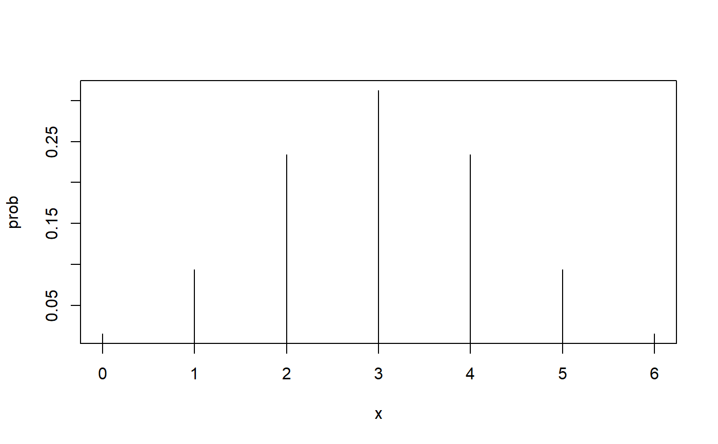
With a little thought, you may recognize that the picture we are looking at here is under some sort of null hypothesis stating that neither fertilizer is more effective than the other. The picture shows the probability of every possible number of positive signs for our difference scores when the sign of the difference is due to chance assignment of fertilizers to trees, but nothing else. It is basically the same distribution we would get if we didn’t use fertilizer at all! In this case, a positive sign would be due to other non-fertilizer-related characteristics of the trees and placement of the trees. We could write a null hypothesis that looks something like this.
Fertilizer doesn’t make a difference
That’s a fine research null hypothesis, but how can we make it a statistical null hypothesis? The key is to think again about our difference scores. Is there any value of any statistic (and associated parameter) that will reflect an equal number of positive and negative difference scores? You probably have guessed that the answer is “yes.” Consider this null hypothesis.
\(H_0: \theta = 0\)
We use \(\theta\) to represent the population median. If the chance of a difference score being positive is the same as the chance of a difference score being negative (that is, the probability of each if 50%), then the median of the difference scores is 0. For our fertilizer research, we can write the null and alternative hypotheses like this.
\(H_0: \theta = 0\)
\(H_a: \theta \ne 0\)
I am using a two-sided alternative here because we went into this study with no information that one fertilizer should be better than the other. The situation would have been different if, for example, we were told that Fertilizer B was developed based on new understanding of the properties of fertilizers so that the research is to confirm that Fertilizer B results in higher production than Fertilizer A.
Let’s set \(\alpha\), our maximum allowable Type I error rate, at 10%. Under the null hypothesis, here is the probability of obtaining only two plus signs for Fertilizer A.
For a two-sided test, we need to also include upper tail values that are equally incompatible with the null hypothesis. That is, we need to include the probability of four or more plus signs among our difference scores. (Notice that four plus signs would be the same as two negative signs for Fertilizer B.)
A p value of 0.6875 will certainly not persuade us to view this as an unlikely outcome, so we must retain a median of 0 as a reasonable possibility for the value of the parameter. Yet we remember that the number of trees with Fertilizer B that outperformed their matched pair tree (not to be confused with a pear tree, which is reserved for partridges) was four out of the six, or 0.67. What gives?
We didn’t have much power for this test because we only used six matched pairs. Let’s see what would happen if we kept the 2 to 1 ratio the same, but used 30 matched pairs. (This would require us to plant 60 trees.) Here’s the picture under the null hypothesis.
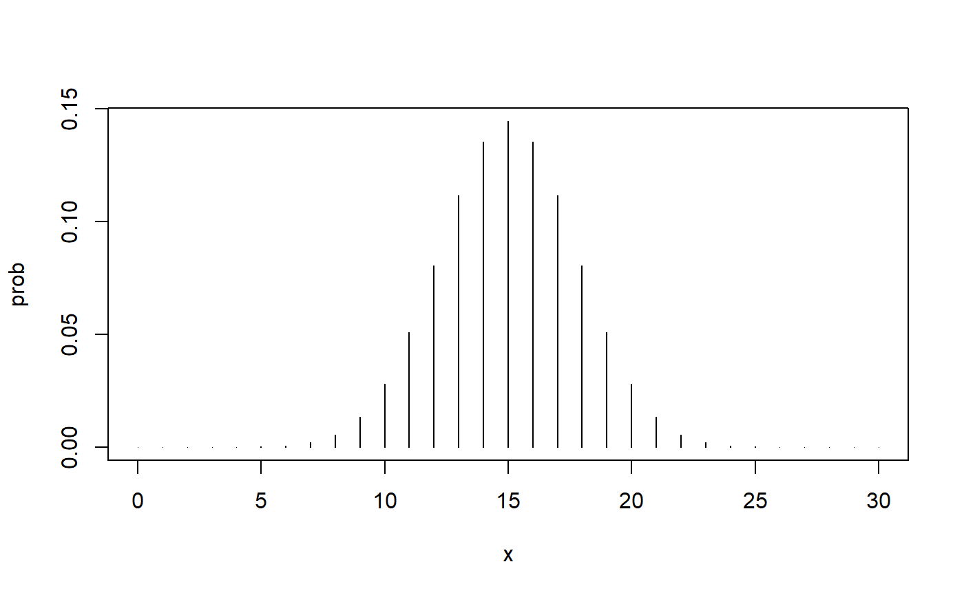
The 2 to 1 ratio would mean that we have 10 plus signs for Fertilizer A and 20 negative signs. Here’s the p value for the two-sided test.
This is better! We have some convincing evidence that Fertilizer B outperforms Fertilizer A. Unlike with some hypotheses you may test with the binomial test, the sign test is always based on a null hypothesis of equal probability (0.5) of plus and minus signs, so the binomial distribution when the null hypothesis is true is symmetrical. Thus, for two-tailed tests it will work to double the probability in one tail when you are calculating the p value.
A confidence interval for the median
Suppose in our fruit tree study that we have reason to believe that the median of difference scores is 1. (I have no idea why we might have a reason to believe this, but stick with me. I’ll put this irrational suspicion to rational use in a moment.) In practical terms, this would mean that the median increase in fruit production is one piece of fruit if Fertilizer B is used instead of Fertilizer A. Similarly, we could propose a median of -1, which would again mean an increase in fruit production, but this time if Fertilizer A is used instead of Fertilizer B.
By definition, the median has 50% of scores above it and 50% of scores beneath it. Therefore, we can test the hypothesis that the median is 1 using the sign test, because the sign test uses a null hypothesis that 50% of the signs are plus signs and 50% of the signs are minus signs. The only difference between this hypothesis test and the hypothesis of no difference in fruit production is that in the earlier hypothesis test, no difference in fruit production corresponded to a median of 0. Thus, we were able to look at the actual sign of each difference. For testing that the median is 1, we need to count any value above 1 as a “plus sign” and any value below 1 as a “minus sign”. This is a bit bizarre, because now we will think of 0 as having a minus sign.
Here are the differences we calculated earlier.
If the median value in the population is 1, then we have 1 value above this median and 4 values below this median. We also have a single value that falls right on the median. How are we going to handle this? One possibility is to just use the 5 values that are either above or below the median, and indeed that is what some statisticians recommend for this situation. This approach is a bit peculiar, because it means that you are throwing out the one data point that is totally consistent with the null hypothesis that the median is 1. That is stacking the deck in favor of the alternative hypothesis!
Let’s calculate the p value two ways. First, we’ll calculate it as if the value of 1 is above the median. Next, we’ll calculate it as if the value of 1 is below the median. Here’s the first way. Remember that we now have two plus signs (“above” 1) and four negative signs (below 1).
That should look familiar. It is the same p value we obtained when testing if the median is equal to 0. That’s no surprise because by counting 1 as “above” the median (even though it is right on the median), we are ending up with the same number of plus and minus signs as before. What happens if we count the 1 as being “below” the median?
That dramatically changed the picture! Neither of these p values will lead us to reject the null hypothesis of a population median of 1, based on our established tolerance for error of 10%, but this second p value gets us much closer to our rejection line. Which of these should we use? Given our distaste for Type I errors and knowing that the value in question is as strongly in support of the null hypothesis as possible (the value is 1 and our hypothesized median is also 1), I recommend that we use the first p value in order to move us further away from rejecting the null hypothesis and more likely to retain it.
If you remember the rule about confidence interval construction, you have probably guessed where this is all going. Let’s review the steps, adding this new rule that we just discussed.
Determine our confidence level. This will correspond to our tolerance for errors in that our confidence level will be \((1 - \alpha)100\%\), where \(\alpha\) is the maximum Type I error rate that we can tolerate.
Hypothesize a median, \(\theta\).
Count how many of the matched pair differences are below the median (call these minus signs) and how many of these differences are above the median (call these plus signs). For a difference that is equal to the hypothesized median, call it either a minus sign or a plus sign, depending on which will make it more difficult to reject the null hypothesis. (Here’s a short cut: when a difference is equal to the hypothesized median, give it a plus or minus sign that will bring the number of plus and minus signs closer to each other, rather than farther away from each other.)
Reject hypotheses in which \(p \le \alpha\). Otherwise, retain the hypothesis.
-
Test all possible hypotheses. Symbolically, we can state it like this.
\(H_0: \theta = \theta_0\)
\(H_1: \theta \ne \theta_0\)
\(-\infty < \theta_0 < +\infty\)
The confidence set consists of all values of \(\theta_0\) that are retained.
If we are interested in whether a median is only above or only below 0 (as we would have been if Fertilizer B was developed to be an improvement on Fertilizer A), then we would test a one-sided hypotheses. Aside from this, the construction of a lower-bounded or upper-bounded interval is the same.
In practice, we will not test every possible \(\theta_0\) because we have other more interesting activities to pursue in life. Instead, we will search for the boundary between rejection and retention. For the above data, let’s test a median of 10. That gives us 1 plus sign and 5 minus signs.
Let’s try these hypotheses.
\(H_0: \theta = 3\)
\(H_1: \theta \ne 3\)
We now have 0 plus signs and 6 negative signs.
We finally have a rejected null hypothesis. We will obtain similar results if we use these hypotheses.
\(H_0: \theta = -13\)
\(H_1: \theta \ne -13\)
Now we have 6 plus signs and 0 negative signs.
You probably noticed that this is the same calculation as the previous one, but with the addends swapped. We have determined that every hypothesized value that yields between 1 and 5 plus (or minus) signs will result in retention. Thus, we are able to define our 90% confidence interval.
\(-12 \le \theta \le 2\)
There are a few elements of this interval construction that are noteworthy. First, we would have obtained the same rejection results if we had hypothesized -14 instead of -13 and 4 instead of 3. Yet we desire the narrowest interval we can obtain, so because -13 and 3 are also rejected, we use -12 and 2 as the first values in our retention region. These become the inclusive boundaries of the confidence interval.
My other comment is a bit more disconcerting. Our testing has wandered outside of the range of our data in order to obtain a 90% confidence interval. That feels a bit like extrapolating beyond the data, so I’m not totally comfortable. That said, it is the best we can do with such a small sample size.
Previously, I provided an example of hypothesis testing with a larger sample size, so it seems in order to do the same for a confidence interval example. The difference here is that we need differences. (Pun only partially intended.) If we want to construct a confidence interval for the median, we need to know more than how many times Fertilizer B beat Fertilizer A. We need to know the extent of this beating by comparing fruit yields.
Here is a (hypothetical) construction of yield differences where I subtracted the yield for A from the yield of the B matched pair tree. Note that I switched the order of subtraction so as to have more positive signs. My only reason for doing this is that I think it makes it easier to teach about an improvement (such as what we are seeing in these data when using Fertilizer B) when the scores are positive.
B.minus.A <- c(-1, 0, -1, 0, 4, 5, 25, 15, 5, 125, 61, 2, 7, -2, 2, 1, 7, 12,
               23, 1, 86, 17, 6, 12, -1, 1, -1, -2, 58, 3, 2, 18, 1, 40, -1,
               2, 12, 0, 3, 6, -2, 1, 56, 5, -2, 8, -2, -1, 30, 1, 2, 52,
               3, -1, 52, 7, 18, 9, 145, 17)
Let’s determine how many matched pairs we have observed and how many plus signs are in these data.
That means there must be 15 values that are either minus signs or 0. (I’m going to leave 0 in with the minus signs to reduce the chance of rejecting the null hypothesis.) Here’s the p value.
I’m quite confident that the fertilizers are not equally effective. Using what we have learned about confidence interval construction, let’s determine an interval for the population median. The previous time we did this, we used a trial and error method to find the number of plus signs that would result in rejection of the null hypothesis. That could be time consuming for larger data sets, such as this one, so let us be a bit more systematic in our approach. This time we will use a 5% error rate so that we can develop a 95% confidence interval. We are using a symmetrical binomial distribution (remember that \(\pi_0 = .5\) for all of our tests), so we can split the error rate into two equal parts and put a proportion of .025 in each tail of the distribution. With this knowledge in hand, we can find the number of plus signs needed to reject the null hypothesis.
We can reject the null hypothesis in the upper tail of the distribution if we have 39 or more plus signs. Similarly, we can reject the null hypothesis in the lower tail of the distribution if we have 39 or more negative signs, which would equate to 60 - 39 = 21 or fewer plus signs. Here’s a check of our work.
Notice what we get if we add one more sign to the rejection region in each tail.
This slightly exceeds our tolerance for Type I errors. Thus, we will use 21 and 39 as our critical values, noting in the process that \(\hat{\alpha} = 0.027\).
The trick now is to find the differences that will result in 21 or fewer plus signs or 39 or more plus signs. Let’s sort our differences. (Not to be confused with “let’s sort out our differences,” though if you are explaining all of this to someone opposed to nonparametric statistical methods, both phrases may apply.)
B.minus.A <- sort(B.minus.A)
B.minus.A
#>  [1]  -2  -2  -2  -2  -2  -1  -1  -1  -1  -1  -1  -1   0   0   0   1   1
#> [18]   1   1   1   1   2   2   2   2   2   3   3   3   4   5   5   5   6
#> [35]   6   7   7   7   8   9  12  12  12  15  17  17  18  18  23  25  30
#> [52]  40  52  52  56  58  61  86 125 145
Now it is easy to find the difference values that sit on our critical values. (Note that if we count from 40 to 60, including 40, there are 21 values, which is why we are taking the 40th value rather than the 39th value.)
We will reject any difference that is greater than or equal to 9 because there are 21 numbers (plus signs) that are 9 or above. Let’s check that.
Similarly we will reject any difference that is less than or equal to 1 because there are 39 numbers (plus signs) above 1. Let’s check that, as well.
Another way to think of this is that we have 21 numbers greater than or equal to 9 (plus signs) and 21 numbers less than or equal to 1 (minus signs).
Either way you prefer to think about it, the point is that we will reject the null hypotheses about the median being 9 or above 9, as well as null hypotheses about the median being 1 or below 1. Further, these values sit right on the edge of the rejection region. The next values in our data set after these, the first ones in our retention region, are 2 and 8. We would retain hypotheses about 2 and 8, as well as any value in between.
\(2 \le \theta \le 8\)
We have now created a 95% confidence interval for the median. In practical terms, this tells us that switching from Fertilizer A to Fertilizer B will result in a median yield increase of 2 to 8 pieces of fruit. (If Fertilizer B is more costly, switching may not be worth it.)
Let’s use these data one more time to construct a one-sided confidence interval for the median difference. This is what we would do if one fertilizer was purposefully developed to be an improvement over the other. The choice of a one-sided interval is not a decision based on the data, but one based on theoretical understanding. Here are the hypotheses.
\(H_0: \theta = 0\)
\(H_A: \theta > 0\)
If the population median is 0, as reflected by the null hypothesis, we would expect the same number of plus and minus signs in our data. If the population median is above 0, as reflected in the alternative hypothesis, we would expect more plus signs than minus signs in our data. Thus, we want to reject the null hypothesis in favor of the alternative hypothesis when there are more plus signs than would be expected by mere chance assignment of our fruit trees. Let’s calculate how many that would be if we want 95% confidence.
We will reject the null hypothesis if we have at least 37 plus signs. We saw earlier that we have 45 plus signs, so we know, with 95% confidence, that the median is above 0. (This is no surprise because our two-sided interval was completely above 0.) Next, let’s use these hypotheses.
\(H_0: \theta = 1\)
\(H_A: \theta > 1\)
Notice that this will reduce the number of plus signs by 6, because there are 6 values of 1 in our data.
We can reject this null hypothesis as well because the observed test statistic, the number of plus signs, is above our critical value of 37 plus signs. Let’s do this one more time with these hypotheses.
\(H_0: \theta = 2\)
\(H_A: \theta > 2\)
We clearly cannot reject this null hypothesis. Notice that the observed value of the test statistic jumped from 39 to 34. That is because we have 5 values of 2 in the data. If we had observed 1 or 2 values of 2, we could have rejected the null hypothesis. As it is, it would be foolhardy to reject the hypothesis based on some of the values of 2 but retain it for others. We must retain the null hypothesis. The consequence of all these values of 2 is that our \(\hat{\alpha}\) has moved away from \(\alpha\). This will yield a less informative interval than we would have had if every fruit yield difference had been unique. In fact, our lower bound is no more informative in this one-sided interval, where we put our entire tolerance for error (5%) in one tail of the distribution, than it was for the two-sided interval. Such is the nature of the real world. Ignoring the effects of worms, fruit yield will be in discrete and whole units, so probabilities are not continuous. As a result, life as a nonparametric statistican can look strange. Keep in mind that the strangeness really resides in the tradition we’ve become used to: Treating discrete numbers as though they are plucked from a continuous distribution. Now that is strange!
Here is our interval.
\(\theta \ge 2\)
You are probably hoping that I’m going to surprise you with a function that will do all of this for us. Surprise! The function is not part of Base R, but it is available in a package written by Andri Signorell. Here it is being used for our two-sided test and interval.
SignTest(B.minus.A)
#>
#>  One-sample Sign-Test
#>
#> data:  B.minus.A
#> S = 45, number of differences = 57, p-value = 1.313e-05
#> alternative hypothesis: true median is not equal to 0
#> 97.3 percent confidence interval:
#>  2 8
#> sample estimates:
#> median of the differences
#>                       4.5
If you go back and look at the p value we calculated for the sign test to test the original number of signs, that is, using the hypothesis that \(\theta = 0\), you will see that it matches with the p value reported by this function, so that’s the meaning of the p value. The confidence interval also matches our two-sided confidence interval. Notice that it is inclusive of the reported boundaries. The function also reports the point estimate, which is the median of differences for our sample and the best single guess of the population median, though without confidence. Let’s see how to obtain the one-sided interval.
SignTest(B.minus.A, alternative = "greater")
#>
#>  One-sample Sign-Test
#>
#> data:  B.minus.A
#> S = 45, number of differences = 57, p-value = 6.564e-06
#> alternative hypothesis: true median is greater than 0
#> 95.4 percent confidence interval:
#>    2 Inf
#> sample estimates:
#> median of the differences
#>                       4.5
The confidence interval is reported as “2 to inf.” The “inf” stands for infinity, which simply means that we have constructed a lower-bounded confidence interval.
Here’s one more little trick with this function. Remember that in our original example we started by recording the amount of fruit picked from each tree, putting matched pairs in the same order for each fertilizer type.
We can use the differences as an argument to the SignTest function, as we did above, or we can provide the measures separately, but in the matched order.
SignTest(fruit$A, fruit$B, conf.level = 0.90)
#>
#>  Dependent-samples Sign-Test
#>
#> data:  fruit$A and fruit$B
#> S = 2, number of differences = 6, p-value = 0.6875
#> alternative hypothesis: true median difference is not equal to 0
#> 96.9 percent confidence interval:
#>  -12   2
#> sample estimates:
#> median of the differences
#>                      -4.5
Conditions for valid inference
As always, calculating correct values is only part of the story when it comes to valid inference. We also must ascertain that our inferential statments are consistent with our research processes. In my experience I have observed that it is quite common for researchers to either make statements about the conditions for valid inference without actually matching each statement to the research process or to ignore the conditions entirely. In either case, statements of inference can be misleading, at best, and potentially dishonest. We must go beyond calculation to put careful thought into what we can and cannot say. The good news is that even when conditions are not completely met, usually our study can still inform practice, even though we may have to curb our enthusiasm about how we report our outcomes.
The first condition for valid inference back to a larger population is that we have randomly sampled from that population. As I’ve discussed before, in the behavioral and social sciences we rarely are able to sample from the entire population of interest, yet a more limited random sampling can still provide use a rationale for inference. Even without random sampling, we can often consider our sample as what we might obtain through random sampling from some population of interest. In the current agriculture setting, it is doubtful that the seeds for these trees were randomly selected from the population of seeds for this particular type of fruit. Yet it is very likely that there is nothing special or specific about these seeds so that they could represent the larger population of seeds, much as if they had been randomly selected.
The second condition for valid inference with the sign test is that the units within each matched pair were randomly assigned (i.e., randomized) to one of the two conditions. This condition is necessary to confirm that it is the explanatory variable, rather than extraneous varibles, responsible for any observed difference. In the present example, if we did not randomize the fruit trees to the fertilizer conditions, then there might be some other condition, such as sun exposure, that could be responsible for differences in production. This could occur without researcher awareness, for levels of extraneous variables can often be undetected in such a study. It could be the case that even with randomization that sun exposure is greater for trees receiving one type of fertilizer, but the randomization process assures us that this is not a systematic bias. The incidence of non-systematic bias is accounted for in our recognized potential for a Type I error, for which we are able to determine our maximum tolerance.
There is one type of study in which random sampling, but not randomization, is key to inference, and that is when the study is not about a treatment effect, but rather is about understanding the characteristics of a single population of scores. In such a case there is no treatment-control comparison, so there are no matched pairs. The sign test can still be used to construct a confidence interval for the median, but in this situation the median of interest is the median of a population of scores, rather than the median of differences. It is also the case that in this single-sample non-experimental situation that the scores can be ordinal (ordered categories), rather than interval (quantitative). Unlike the mean, the median is a valid indicator of central tendency with ordinal data. In a randomized experiment, however, the use of difference scores requires that our measures be quantitative. That is, the data must be at least interval.
It is possible to make inferences when you use a matched-pair design with a randomized experiment and only make ordinal measurements. In this situation the process involves determining a “winner” in each matched pair. A win in one direction is counted as a plus sign, while a win in the other direction is counted as a minus sign. The sign test can then be employed to determine if we can infer that a favorable outcome for one condition is evidence of treatment effectiveness. This is a single hypothesis test as we are unable to conduct multiple tests of median difference, so we cannot construct a confidence interval.
The third condition for valid inference is that matched pairs are independent of one another. Measures within pairs are not independent of each other. Indeed, they have been purposefully matched on various characteristics related to the variable of interest. Yet each pair should be independent of each other pair. In the present example, this was assured through using separate planting areas for each pair of fruit trees.
If you read about the sign test from other sources, you will freqently encounter a fourth condition. Namely, that scores must be continous. The purpose of this condition is to guarantee that a plus or minus sign will be available for every difference. If values are truly continuous, they will never be equal, so this will indeed ensure that every difference is associated with a sign. In reality, however, we use discerete measurement. Thus, we may declare a matched pair to be equivalent on our measure. If a “winner” can be declared, we can avoid such ties. If not, the methods described above will yield tests and intervals that control our Type I error rate. The consequence of ties will be a more conservative test or confidence interval.
For those who are new to nonparametric inference, it may seem unusual to use the median, rather than the mean, as the central tendency parameter. If this seems strange, it is because the mean is ubiquitous in parametric inference. Yet the median is a strong contendor as a measure of central tendency with desirable properties. Among these is an insensitivity to outliers that can be overly influential on the mean. Further, when the population is symetrical, the values of the mean and the median are the same. This equivalency suggests that if we add a condition of symmetry, we can build a confidence interval for the mean, rather than the median. This is true, though I recommend that we dispense with this additional condition and build intervals for the population median. I see no advantage in creating a confidence interval for the mean, other than to maintain friendships with those who choose to invest all of their energies in parametric inference. Even in those cases, we may be able to keep both our median-oriented confidence intervals and our friendships if we consider additional procedures, such as buying after-work drinks or bringing in doughnuts.
Let me end this discussion about the conditions for valid inference by considering those conditions we grew up with when we first learned about parametric inference. With a matched-pair design, we were able to test the following hypotheses.
\(H_0: \mu = \mu_0\)
\(H_a: \mu \ne \mu_0\)
Here, \(\mu_0\) is a specific null hypothesis. By considering all values for this hypothesis, we were able to build a confidence interval for the mean. The conditions for valid inference in this setting are those listed above (random sample, randomization, and independence of matched pairs), plus an additional condition that the differences calculated for comparing our treatment-control pairs is normally distributed. This last assumption is referred to as a strong condition. The term strong does not mean it is a valuable condition, but that it is a more strict condition than the others. With the sign test for a median, we can dispense with strong conditions. If we desire a confidence interval for the mean, rather than the median, then we must consider the strong condition that differences scores are symmetrical. This is more difficult to ascertain than the other conditions, yet the condition is still not as strong as the requirement that the differences scores are normally distributed.
A test for trend
In 1955, D. R. Cox and A. Stuart published an article in Biometrika in which they suggested using the sign test for a test of trend. Their method is simple. They compared the first half of ordered scores to the second half by taking each measure in the first half and comparing it to a corresponding measure in the second half. When the second half measure exceeded that of the first half, they designated that as a plus sign. If not, they designated it as a minus sign.
Here are the average global land-ocean temperatures for the years 1999 through 2018 (Source: NASA’s Goddard Institute for Space Studies).
year <- c(1999:2018)
temp <- c(0.39, 0.40, 0.54, 0.63, 0.63, 0.54, 0.68, 0.64, 0.67, 0.55, 0.66,
          0.73, 0.61, 0.65, 0.69, 0.75, 0.90, 1.02, 0.93, 0.85)
cbind(year, temp)
#>       year temp
#>  [1,] 1999 0.39
#>  [2,] 2000 0.40
#>  [3,] 2001 0.54
#>  [4,] 2002 0.63
#>  [5,] 2003 0.63
#>  [6,] 2004 0.54
#>  [7,] 2005 0.68
#>  [8,] 2006 0.64
#>  [9,] 2007 0.67
#> [10,] 2008 0.55
#> [11,] 2009 0.66
#> [12,] 2010 0.73
#> [13,] 2011 0.61
#> [14,] 2012 0.65
#> [15,] 2013 0.69
#> [16,] 2014 0.75
#> [17,] 2015 0.90
#> [18,] 2016 1.02
#> [19,] 2017 0.93
#> [20,] 2018 0.85
To use the Cox-Stuart test for trend, we will compare first half temperatures to those in the second half. We will compare 1999 to 2009, 2000 to 2010, 2001 to 2011, and so on. Whenever the second half temperature is greater than the first half comparison, we will designate this as a plus sign. Otherwise, we will designate it as a minus sign.
first.half <- temp[1:10]
second.half <- temp[11:20]
plus.sign <- second.half > first.half
sum(plus.sign)
#> [1] 10
With this first half comparison to the second half, the null hypothesis of no trend is that the probability of the second half value being greater than the first half value is 0.5.
\(H_0: \pi_{2nd} = \pi_{1st}\)
\(H_A: \pi_{2nd} > \pi_{1st}\)
Using the global temperature data, here is the test using \(\alpha = .05\).
binom.test(10, 10, 0.5, alternative = "greater", conf.level = 0.95)
#>
#>  Exact binomial test
#>
#> data:  10 and 10
#> number of successes = 10, number of trials = 10, p-value =
#> 0.0009766
#> alternative hypothesis: true probability of success is greater than 0.5
#> 95 percent confidence interval:
#>  0.7411344 1.0000000
#> sample estimates:
#> probability of success
#>                      1
There is strong evidence of a global warming trend.