Replacement Scores
ReplaceScores.RmdWe can conduct a matched-pair randomization test using only the sign of the differences, or we can also consider the magnitude of the difference. We can also replace the magnitude of the difference with another score that is related to this magnitude such that the order or sign of the differences are not changed. In this vignette we will discuss two possible replacement scores and examine some reasons why we might want to replace our original measures of the magnitude of a difference.
The Wilcoxon signed ranks test
A disadvantage of the Fisher-Pitman permutation test is that with even moderately-sized samples the number of possible permutations can grow large so that calculations are prohibitive. Let’s look at a little table showing the number of differences and the number of possible permutations associated with that number of differences.
differences <- 2:50
num.perms <- 2^differences
noquote(cbind(differences, format(num.perms, scientific = FALSE)))
#>       differences
#>  [1,] 2                          4
#>  [2,] 3                          8
#>  [3,] 4                         16
#>  [4,] 5                         32
#>  [5,] 6                         64
#>  [6,] 7                        128
#>  [7,] 8                        256
#>  [8,] 9                        512
#>  [9,] 10                      1024
#> [10,] 11                      2048
#> [11,] 12                      4096
#> [12,] 13                      8192
#> [13,] 14                     16384
#> [14,] 15                     32768
#> [15,] 16                     65536
#> [16,] 17                    131072
#> [17,] 18                    262144
#> [18,] 19                    524288
#> [19,] 20                   1048576
#> [20,] 21                   2097152
#> [21,] 22                   4194304
#> [22,] 23                   8388608
#> [23,] 24                  16777216
#> [24,] 25                  33554432
#> [25,] 26                  67108864
#> [26,] 27                 134217728
#> [27,] 28                 268435456
#> [28,] 29                 536870912
#> [29,] 30                1073741824
#> [30,] 31                2147483648
#> [31,] 32                4294967296
#> [32,] 33                8589934592
#> [33,] 34               17179869184
#> [34,] 35               34359738368
#> [35,] 36               68719476736
#> [36,] 37              137438953472
#> [37,] 38              274877906944
#> [38,] 39              549755813888
#> [39,] 40             1099511627776
#> [40,] 41             2199023255552
#> [41,] 42             4398046511104
#> [42,] 43             8796093022208
#> [43,] 44            17592186044416
#> [44,] 45            35184372088832
#> [45,] 46            70368744177664
#> [46,] 47           140737488355328
#> [47,] 48           281474976710656
#> [48,] 49           562949953421312
#> [49,] 50          1125899906842624
Even with 50 difference scores we are into territory where calculation time might become a factor. I’m going to make the assumption that we can do the calculations for 10,000,000 permutations per second.
Although 3.6 years might seem worth it for a study of high scientific value, we wouldn’t want to do this too often. If we repeat the study with a different set of numbers, we have to do the calculations all over again. (Can you imagine being about two years into your wait for the calculations to be done when you suddenly discover a typo in your data set?!)
One solution to the problem is to replace our original scores with ranks. Just as with the Fisher-Pitman permutation test, we order the scores (now we will use ranks instead of scores) without regard to the observed sign. Once we have done this, we can then look at all possible permutations of signs. We again use the sum of the positive scores (i.e., ranks) as our test statistic. As it is when we use scores, and using the same hypotheses, if the null hypothesis is true, we expect the sum of positive ranks to equal the sum of negative ranks, but with opposite signs. If the null hypothesis is not true, we would expect the sum of positive ranks to become either larger or smaller than we would expect.
Here are the data from the fertilizer study.
fruit <- data.frame(A = c(82, 91, 74, 90, 66, 81),
                    B = c(85, 89, 81, 96, 65, 93))

cbind(fruit$A, fruit$B)
#>      [,1] [,2]
#> [1,]   82   85
#> [2,]   91   89
#> [3,]   74   81
#> [4,]   90   96
#> [5,]   66   65
#> [6,]   81   93
A.minus.B <- fruit$A - fruit$B
A.minus.B
#> [1]  -3   2  -7  -6   1 -12
Here are the ranks for these data, without regard to sign.
Now let’s attach signs to them.
Our test statistic is the sum of positive ranks.
Let’s look at the distrbution of the test statistic when the null hypothesis is true. Notice that we are doing just what we did for the Fisher-Pitman test, but this time we are using ranks instead of the original scores.
rand_dist(fruit.rank)
#>       T
#>  [1,] 0  0.0156250 0.0156250 1.0000000
#>  [2,] 1  0.0156250 0.0312500 0.9843750
#>  [3,] 2  0.0156250 0.0468750 0.9687500
#>  [4,] 3  0.0156250 0.0625000 0.9531250
#>  [5,] 3  0.0156250 0.0781250 0.9375000
#>  [6,] 4  0.0156250 0.0937500 0.9218750
#>  [7,] 4  0.0156250 0.1093750 0.9062500
#>  [8,] 5  0.0156250 0.1250000 0.8906250
#>  [9,] 5  0.0156250 0.1406250 0.8750000
#> [10,] 5  0.0156250 0.1562500 0.8593750
#> [11,] 6  0.0156250 0.1718750 0.8437500
#> [12,] 6  0.0156250 0.1875000 0.8281250
#> [13,] 6  0.0156250 0.2031250 0.8125000
#> [14,] 6  0.0156250 0.2187500 0.7968750
#> [15,] 7  0.0156250 0.2343750 0.7812500
#> [16,] 7  0.0156250 0.2500000 0.7656250
#> [17,] 7  0.0156250 0.2656250 0.7500000
#> [18,] 7  0.0156250 0.2812500 0.7343750
#> [19,] 8  0.0156250 0.2968750 0.7187500
#> [20,] 8  0.0156250 0.3125000 0.7031250
#> [21,] 8  0.0156250 0.3281250 0.6875000
#> [22,] 8  0.0156250 0.3437500 0.6718750
#> [23,] 9  0.0156250 0.3593750 0.6562500
#> [24,] 9  0.0156250 0.3750000 0.6406250
#> [25,] 9  0.0156250 0.3906250 0.6250000
#> [26,] 9  0.0156250 0.4062500 0.6093750
#> [27,] 9  0.0156250 0.4218750 0.5937500
#> [28,] 10 0.0156250 0.4375000 0.5781250
#> [29,] 10 0.0156250 0.4531250 0.5625000
#> [30,] 10 0.0156250 0.4687500 0.5468750
#> [31,] 10 0.0156250 0.4843750 0.5312500
#> [32,] 10 0.0156250 0.5000000 0.5156250
#> [33,] 11 0.0156250 0.5156250 0.5000000
#> [34,] 11 0.0156250 0.5312500 0.4843750
#> [35,] 11 0.0156250 0.5468750 0.4687500
#> [36,] 11 0.0156250 0.5625000 0.4531250
#> [37,] 11 0.0156250 0.5781250 0.4375000
#> [38,] 12 0.0156250 0.5937500 0.4218750
#> [39,] 12 0.0156250 0.6093750 0.4062500
#> [40,] 12 0.0156250 0.6250000 0.3906250
#> [41,] 12 0.0156250 0.6406250 0.3750000
#> [42,] 12 0.0156250 0.6562500 0.3593750
#> [43,] 13 0.0156250 0.6718750 0.3437500
#> [44,] 13 0.0156250 0.6875000 0.3281250
#> [45,] 13 0.0156250 0.7031250 0.3125000
#> [46,] 13 0.0156250 0.7187500 0.2968750
#> [47,] 14 0.0156250 0.7343750 0.2812500
#> [48,] 14 0.0156250 0.7500000 0.2656250
#> [49,] 14 0.0156250 0.7656250 0.2500000
#> [50,] 14 0.0156250 0.7812500 0.2343750
#> [51,] 15 0.0156250 0.7968750 0.2187500
#> [52,] 15 0.0156250 0.8125000 0.2031250
#> [53,] 15 0.0156250 0.8281250 0.1875000
#> [54,] 15 0.0156250 0.8437500 0.1718750
#> [55,] 16 0.0156250 0.8593750 0.1562500
#> [56,] 16 0.0156250 0.8750000 0.1406250
#> [57,] 16 0.0156250 0.8906250 0.1250000
#> [58,] 17 0.0156250 0.9062500 0.1093750
#> [59,] 17 0.0156250 0.9218750 0.0937500
#> [60,] 18 0.0156250 0.9375000 0.0781250
#> [61,] 18 0.0156250 0.9531250 0.0625000
#> [62,] 19 0.0156250 0.9687500 0.0468750
#> [63,] 20 0.0156250 0.9843750 0.0312500
#> [64,] 21 0.0156250 1.0000000 0.0156250
Let’s clean up the table a bit by combining redundant values.
rand_dist(fruit.rank, show.all = FALSE)
#>       T
#>  [1,] 0  0.0156250 0.0156250 1.0000000
#>  [2,] 1  0.0156250 0.0312500 0.9843750
#>  [3,] 2  0.0156250 0.0468750 0.9687500
#>  [4,] 3  0.0312500 0.0781250 0.9531250
#>  [5,] 4  0.0312500 0.1093750 0.9218750
#>  [6,] 5  0.0468750 0.1562500 0.8906250
#>  [7,] 6  0.0625000 0.2187500 0.8437500
#>  [8,] 7  0.0625000 0.2812500 0.7812500
#>  [9,] 8  0.0625000 0.3437500 0.7187500
#> [10,] 9  0.0781250 0.4218750 0.6562500
#> [11,] 10 0.0781250 0.5000000 0.5781250
#> [12,] 11 0.0781250 0.5781250 0.5000000
#> [13,] 12 0.0781250 0.6562500 0.4218750
#> [14,] 13 0.0625000 0.7187500 0.3437500
#> [15,] 14 0.0625000 0.7812500 0.2812500
#> [16,] 15 0.0625000 0.8437500 0.2187500
#> [17,] 16 0.0468750 0.8906250 0.1562500
#> [18,] 17 0.0312500 0.9218750 0.1093750
#> [19,] 18 0.0312500 0.9531250 0.0781250
#> [20,] 19 0.0156250 0.9687500 0.0468750
#> [21,] 20 0.0156250 0.9843750 0.0312500
#> [22,] 21 0.0156250 1.0000000 0.0156250
As we would expect, the highest probability under the null hypothesis is smack in the middle of the distribution: 10 and 11. We observed a value of 3. If we use a maximum Type I error rate of 0.10 (a confidence level of 90%), we are unable to reject this null hypothesis in favor of this alternative hypothesis.
\(H_0: \theta_d = 0\)
\(H_a: \theta_d \ne 0\)
If we had been conducting a confirmatory test that Fertilizer B included improvements that we expected would make it more effective, we would use these hypotheses.
\(H_0: \theta_d = 0\)
\(H_a: \theta_d < 0\)
In this case, with a maximum Type I error rate of 0.10, we would be able to reject the null hypothesis in favor of the alternative hypothesis. Note that the direction of the alternative hypothesis is determined by the direction of subtraction in order to obtain our difference scores.
So what advantage have we gained by using ranks instead of the observed differences? There are several, but we will discuss one of these right now and hold off on the others for later discussion. Recall our 3.6 year wait for obtaining the distribution when we have 50 paired differences? Using the Wilcoxon signed rank test, we only have to do that once. Why? Because everytime we have 50 paired differences, the ranks will be the same. So one 3.6 year wait is all that we need to compute the distribution of the test statistic that can then be used for all time. We might envision running a bunch of computers for several years, using different sample sizes, and then publishing these distributions. In fact, that’s been done! You and I don’t have to wait.
We have a function in R that can do the Wilcoxon test for us, so let’s use it. Note that we don’t have to convert to ranks first because it will do that for us.
wilcox.test(A.minus.B)
#>
#>  Wilcoxon signed rank test
#>
#> data:  A.minus.B
#> V = 3, p-value = 0.1563
#> alternative hypothesis: true location is not equal to 0
The p value is what we obtained above. Yay!
We can also provide the observations from the separate fruit trees, but be careful. There is also a Wilcoxon test for two independent samples and that’s not what we want here. We need to specify that we want a paired test. When you enter two sets of observations, the default is a two-sample test calculation.
wilcox.test(fruit$A, fruit$B, paired = TRUE)
#>
#>  Wilcoxon signed rank test
#>
#> data:  fruit$A and fruit$B
#> V = 3, p-value = 0.1563
#> alternative hypothesis: true location shift is not equal to 0
We can, of course, use this for a one-sided test.
wilcox.test(fruit$A, fruit$B, paired = TRUE, alternative = "less")
#>
#>  Wilcoxon signed rank test
#>
#> data:  fruit$A and fruit$B
#> V = 3, p-value = 0.07813
#> alternative hypothesis: true location shift is less than 0
What about if we use very large sample sizes? In that case, the function will switch to an approximation. (We will discuss large-sample approximations later.) It uses 50 as the cut-off. Up to 50, it will use an exact test. For 50 and over, it will use an approximation. We can force an exact test in these larger sample settings, but will it work? Let’s try it.
# Obtain 60 observations from trees with Fertilizer A. I'm going to assume that
# these observations are normally distributed.

large.A <- rnorm(60, mean = 80, sd = 10)

# Do it again for Fertilizer B. I'm going to assume that we obtain an average
# of 3 more bushels of fruit from this tree.

large.B <- rnorm(60, mean = 83, sd = 10)

# Let's suppose we are doing confirmatory research, so we'll do a one-sided
# test. Now we hold our breath and hope that we aren't holding it for 400
# years.

wilcox.test(large.A, large.B, paired = TRUE, alternative = "less", exact = TRUE)
#>
#>  Wilcoxon signed rank test
#>
#> data:  large.A and large.B
#> V = 614, p-value = 0.01311
#> alternative hypothesis: true location shift is less than 0
Wow! It did it, and fast! Let’s see how this compares to if we had just let the function do the large-sample approximation.
wilcox.test(large.A, large.B, paired = TRUE, alternative = "less")
#>
#>  Wilcoxon signed rank test with continuity correction
#>
#> data:  large.A and large.B
#> V = 614, p-value = 0.01348
#> alternative hypothesis: true location shift is less than 0
This is quite good, which is why the function switches to the large-sample approximation at 50. We know that the Fisher-Pitman permutation test with original scores would take way too long for us to do in our lifetime. (Maybe grandchildren could get our results off the printer and help establish our lebacy!) Yet we also know that the t test is a large-sample approxiamation for the Fisher-Pitman permutation test, so let’s see how those results compare.
t.test(large.A, large.B, paired = TRUE, alternative = "less")
#>
#>  Paired t-test
#>
#> data:  large.A and large.B
#> t = -2.4673, df = 59, p-value = 0.008267
#> alternative hypothesis: true difference in means is less than 0
#> 95 percent confidence interval:
#>       -Inf -1.296225
#> sample estimates:
#> mean of the differences
#>               -4.016758
Remember that we simulated this study using random numbers, so your results will be different than mine, and my results will be different every time I go through this vignette. What we do know is that most of the time we should obtain a smaller p value with the t test. Why? Because we have exactly met the conditions for valid inference with the t test by simulating our data using a normal distribution. I will venture, however, that most of the time when you try this with normally distributed data that your results will not differ too drastically from what you are obtaining with the Wilcoxon test. This is surprising given that the t test is valid, and most powerful, when the sample comes from a normal distribution. We will discuss this further when we compare the power of competing methods.
Conditions for valid inference
When we used original scores, rather than ranks, the permutation test was the Fisher-Pitman permutation test. Here are the conditions for valid inference we needed with the Fisher-Pitman test.
- The sample is randomly drawn from the population of interest.
- Pairs must be independent of one another.
- The scale of measurement is interval.
- The differences obtained within pairs are symmetrically distributed across pairs. This last condition can be achieved with randomization of pair members to the treatment and control conditions.
The conditions for valid inference with the Wilcoxon signed ranks test are the same as those for the Fisher-Pitman permutation test. This leads to an obvious question: Which should we use? Above we saw that we can use the Wilcoxon method for sample sizes that are too large for the Fisher-Pitman permutation method, at least in our lifetimes. Later we will answer the question for situations in which both methods are possible.
The “problem” of ties
I am going back to our original fertilizer example, but I’m going to alter the scores a bit so that you can see how it creates a “problem.”
fruit$A2 <- c(82, 91, 74, 90, 66, 81)
fruit$B2 <- c(85, 89, 80, 96, 65, 93)
A2.minus.B2 <- fruit$A2 - fruit$B2
cbind(fruit$A2, fruit$B2, A2.minus.B2)
#>            A2.minus.B2
#> [1,] 82 85          -3
#> [2,] 91 89           2
#> [3,] 74 80          -6
#> [4,] 90 96          -6
#> [5,] 66 65           1
#> [6,] 81 93         -12
Only one value changed slightly, yet this one change means that we have a tie among our difference scores. Why is this important? If we are going to rank the absolute value of the differences, as is required for the Wilcoxon method, how do we rank the two values of -6? (Note that we would have also had a tie if one of these was -6 and one was 6, because we rank the absolute values of the scores.)
At least three methods have been proposed for dealing with ties. These are:
Eliminate the tied values Randomly assign the two ranks to the tied values *Use midranks
The first of these options runs counter to a major pillar of science: Gather as much information as you can to better understand variable relationships. Throwing out data is rather distasteful. From a statistical point of view, we are not going to be happy about taking an already small sample of six pairs and throwing out one-third of the data to leave us with four pairs.
Although the second method retains the data, it also means that two researchers with the exact same scores can arrive at two different results because they some of their results are due to chance outcomes. Although randomness is a powerful tool for both sampling and experimentation, we do not want to randomly select our findings, yet that is what we are doing if we randomly assign ranks and then use a statistical method based on ranking.
The third option addresses all of the concerns of the first two methods. All the data are retained and rankings are not left to chance. A midrank is simply the average of the ranks that would have been assigned to the scores if they were slightly different from each other. For example, look at the ranks that we assigned with our original fruit data.
cbind(A.minus.B, abs.fruit.rank)
#>      A.minus.B abs.fruit.rank
#> [1,]        -3              3
#> [2,]         2              2
#> [3,]        -7              5
#> [4,]        -6              4
#> [5,]         1              1
#> [6,]       -12              6
The values of -6 and -7 received the ranks of 4 and 5, respectively. Now that the value of -7 has changed to -6, we still want to use the ranks of 4 and 5 because those are the correct ranks in the context of the other scores. Yet rather than throwing out or randomly assigning these ranks, we average them and assign this average to both values. The ranking function in R accomplishes this task for us.
We can look at the distribution of sums of all possible positive ranks, just as we did when we did not have ties.
rand_dist(fruit2.rank, show.all = FALSE)
#>       T
#>  [1,] 0    0.0156250 0.0156250 1.0000000
#>  [2,] 1    0.0156250 0.0312500 0.9843750
#>  [3,] 2    0.0156250 0.0468750 0.9687500
#>  [4,] 3    0.0312500 0.0781250 0.9531250
#>  [5,] 4    0.0156250 0.0937500 0.9218750
#>  [6,] 4.5  0.0312500 0.1250000 0.9062500
#>  [7,] 5    0.0156250 0.1406250 0.8750000
#>  [8,] 5.5  0.0312500 0.1718750 0.8593750
#>  [9,] 6    0.0312500 0.2031250 0.8281250
#> [10,] 6.5  0.0312500 0.2343750 0.7968750
#> [11,] 7    0.0156250 0.2500000 0.7656250
#> [12,] 7.5  0.0625000 0.3125000 0.7500000
#> [13,] 8    0.0156250 0.3281250 0.6875000
#> [14,] 8.5  0.0312500 0.3593750 0.6718750
#> [15,] 9    0.0468750 0.4062500 0.6406250
#> [16,] 9.5  0.0312500 0.4375000 0.5937500
#> [17,] 10   0.0312500 0.4687500 0.5625000
#> [18,] 10.5 0.0625000 0.5312500 0.5312500
#> [19,] 11   0.0312500 0.5625000 0.4687500
#> [20,] 11.5 0.0312500 0.5937500 0.4375000
#> [21,] 12   0.0468750 0.6406250 0.4062500
#> [22,] 12.5 0.0312500 0.6718750 0.3593750
#> [23,] 13   0.0156250 0.6875000 0.3281250
#> [24,] 13.5 0.0625000 0.7500000 0.3125000
#> [25,] 14   0.0156250 0.7656250 0.2500000
#> [26,] 14.5 0.0312500 0.7968750 0.2343750
#> [27,] 15   0.0312500 0.8281250 0.2031250
#> [28,] 15.5 0.0312500 0.8593750 0.1718750
#> [29,] 16   0.0156250 0.8750000 0.1406250
#> [30,] 16.5 0.0312500 0.9062500 0.1250000
#> [31,] 17   0.0156250 0.9218750 0.0937500
#> [32,] 18   0.0312500 0.9531250 0.0781250
#> [33,] 19   0.0156250 0.9687500 0.0468750
#> [34,] 20   0.0156250 0.9843750 0.0312500
#> [35,] 21   0.0156250 1.0000000 0.0156250
Here is the sum of positive ranks with our new fruit data.
Looking at 3 in the distribution, we can calculate our p value.
The use of midranks makes so much sense and is the recommended method by many prominent nonparametric statisticians. So why are the other two methods even considered? Let’s see what happens when we use the Wilcoxon test function with these data.
wilcox.test(A2.minus.B2, exact = TRUE, conf.level = 0.90)
#> Warning in wilcox.test.default(A2.minus.B2, exact = TRUE, conf.level =
#> 0.9): cannot compute exact p-value with ties
#>
#>  Wilcoxon signed rank test with continuity correction
#>
#> data:  A2.minus.B2
#> V = 3, p-value = 0.1411
#> alternative hypothesis: true location is not equal to 0
The function doesn’t work! It provides a p value, but this is a large-sample approximation, and obviously we don’t have a large sample. (Though, admittedly, that p value is not very far off.) The algorithm for the exact test that is programmed into many major statistical software packages assumes that there are no ties. Indeed, you can find textbooks that add a condition of either no ties or continuous data (so that you can’t have ties) as a condition for valid inference. Yet we have just seen with our distribution that this condition is not necessary. Fortunately, we are using R and can access many additional functions that are not programmed into base R. Let’s see what the coin package does if we provide it these tied values. The coin package has a function for the Wilcoxon signed ranks test.
wilcoxsign_test(fruit$A2 ~ fruit$B2, distribution = "exact")
#>
#>  Exact Wilcoxon-Pratt Signed-Rank Test
#>
#> data:  y by x (pos, neg)
#>   stratified by block
#> Z = -1.5768, p-value = 0.1562
#> alternative hypothesis: true mu is not equal to 0
That’s the same p value we obtained. Yes! Notice this is now called the Wilcoxon-Pratt test. That’s because Wilcoxon assumed no ties, but back in 1959, Pratt realized that you could use a distribution that includes midranks, just like we did, so that is implemented into the coin algorithm.
Let’s see if this can handle a larger problem, such as the one we looked at above. This time I’m going to round the numbers so that we have a good chance of getting tied ranks.
# Obtain 60 observations from trees with Fertilizer A. I'm going to assume that
# these observations are normally distributed.

large.A <- round(rnorm(60, mean = 80, sd = 10))

# Do it again for Fertilizer B. I'm going to assume that we obtain an average
# of 3 more bushels of fruit from this tree.

large.B <- round(rnorm(60, mean = 83, sd = 10))

# Let's see if we have any ties.

rank(abs(large.B - large.A))
#>  [1] 40.5 52.5 57.0  6.5 36.0 58.5 30.5 40.5 30.5 46.0 36.0 55.0 38.0 30.5
#> [15] 46.0 13.0 44.0 20.0 25.0 25.0 20.0  6.5 30.5 36.0 30.5 55.0  6.5 60.0
#> [29] 40.5 20.0 10.0 49.0 20.0 20.0  6.5  1.5  3.5 30.5 52.5 48.0 20.0 43.0
#> [43] 40.5 46.0 50.5 55.0 50.5 15.5 10.0 30.5 15.5  1.5 25.0 13.0 30.5 13.0
#> [57] 10.0 20.0  3.5 58.5
Now let’s see if the function works for us. Remember we did a one-sided test for this example.
wilcoxsign_test(large.B ~ large.A,
                distribution = "exact",
                alternative = "greater")
#>
#>  Exact Wilcoxon-Pratt Signed-Rank Test
#>
#> data:  y by x (pos, neg)
#>   stratified by block
#> Z = 1.72, p-value = 0.0429
#> alternative hypothesis: true mu is greater than 0
Let’s see how this p value compares to that of the t test.
t.test(large.B - large.A, alternative = "greater")
#>
#>  One Sample t-test
#>
#> data:  large.B - large.A
#> t = 1.7831, df = 59, p-value = 0.03986
#> alternative hypothesis: true mean is greater than 0
#> 95 percent confidence interval:
#>  0.1999369       Inf
#> sample estimates:
#> mean of x
#>  3.183333
Pretty close!
A confidence interval for the median
We have already seen how to construct a confidence interval for the median using the sign test. If we have symmetry, as we do when we use matched pairs and randomize to conditions, we can obtain a narrower interval by constructing a confidence interval using the Wilcoxon test.
Walsh averages
The first step in confidence interval construction is to construct Walsh averages. A Walsh average is the average of a pair of scores. We will need to construct all Walsh averages for all pairs of difference scores. Let’s use our small fertilizer data set as an example. Here is a matrix of Walsh averages.
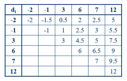
Figure 1
The Hodges-Lehmann median estimate
Hodges and Lehmann showed that the median of Walsh averages is an estimate of the median of scores with strong statistical properties. Thus, in this example, here is the estimate of the median.
median(c(-2, -1.5, -1, 0.5, 1, 3, 2, 2.5, 4.5, 6, 2.5, 3, 5, 6.5, 7,
         5, 5.5, 7.5, 9, 9.5, 12))
#> [1] 4.5
This is a point estimate, which is useful information, but we seek an interval estimate that has an associated level of confidence. Look again at the distribution of the possible sum of positive ranks.
rand_dist(c(1, 2, 3, 4, 5, 6), show.all = FALSE)
#>       T
#>  [1,] 0  0.0156250 0.0156250 1.0000000
#>  [2,] 1  0.0156250 0.0312500 0.9843750
#>  [3,] 2  0.0156250 0.0468750 0.9687500
#>  [4,] 3  0.0312500 0.0781250 0.9531250
#>  [5,] 4  0.0312500 0.1093750 0.9218750
#>  [6,] 5  0.0468750 0.1562500 0.8906250
#>  [7,] 6  0.0625000 0.2187500 0.8437500
#>  [8,] 7  0.0625000 0.2812500 0.7812500
#>  [9,] 8  0.0625000 0.3437500 0.7187500
#> [10,] 9  0.0781250 0.4218750 0.6562500
#> [11,] 10 0.0781250 0.5000000 0.5781250
#> [12,] 11 0.0781250 0.5781250 0.5000000
#> [13,] 12 0.0781250 0.6562500 0.4218750
#> [14,] 13 0.0625000 0.7187500 0.3437500
#> [15,] 14 0.0625000 0.7812500 0.2812500
#> [16,] 15 0.0625000 0.8437500 0.2187500
#> [17,] 16 0.0468750 0.8906250 0.1562500
#> [18,] 17 0.0312500 0.9218750 0.1093750
#> [19,] 18 0.0312500 0.9531250 0.0781250
#> [20,] 19 0.0156250 0.9687500 0.0468750
#> [21,] 20 0.0156250 0.9843750 0.0312500
#> [22,] 21 0.0156250 1.0000000 0.0156250
There’s something interesting to note. The maximum possible sum of ranks is 21, which also happens to be the number of Walsh averages. Coincidence? No! This is always the case, and this knowledge leads to a simple method of confidence interval construction. Note in our distribution that we will reject (at the 90% confidence level) for values less than, or equal to, 2. We can translate this onto our chart of Walsh averages by rejecting the 2 lowest values and the 2 highest values in our table, then putting all other values in the confidence interval. This provides the following interval.
\(-1 \le \theta \le 9\)
Here is the calculation using the wilcox.test function.
wilcox.test(A.minus.B,
            alternative = "two.sided",
            conf.int = TRUE,
            conf.level = 0.90)
#>
#>  Wilcoxon signed rank test
#>
#> data:  A.minus.B
#> V = 3, p-value = 0.1563
#> alternative hypothesis: true location is not equal to 0
#> 90 percent confidence interval:
#>  -9  1
#> sample estimates:
#> (pseudo)median
#>           -4.5
The subtraction was in the opposite direction of ours, but this is no matter as long as we interpret based on direction. Let’s compare it to the interval using the sign test.
SignTest(A.minus.B, conf.level = 0.90)
#>
#>  One-sample Sign-Test
#>
#> data:  A.minus.B
#> S = 2, number of differences = 6, p-value = 0.6875
#> alternative hypothesis: true median is not equal to 0
#> 96.9 percent confidence interval:
#>  -12   2
#> sample estimates:
#> median of the differences
#>                      -4.5
This is wider than the interval we obtained with the Wilcoxon method, which is to be expected when the data are symmetrical. If the data were normal, we could obtain an even narrower interval with the t test, but we shouldn’t go there unless we know we have normally distributed data.
The normal scores test
Although ranks are among the most common replacement scores that we can use to test a hypothesis of interest, there are other possible replacement scores, including those that have a primary advantage of ranks; namely, that the scores are the same for every sample of the same sample size. The reason we should entertain the possibility of alternative replacement scores is that such scores may provide us more power for some distributions of the original scores. I will discuss that in more detail later. For now, let’s look at another type of replacement scores: normal scores.
In the early 1950s, the Dutch mathematician Bartel Leender van der Waerden proposed replacing scores with quantiles of the normal distribution and developed some statistical tests using these replacement scores. In honor of this insight, we refer to these as van der Waerden normal scores. Here is a picture to illustrate how we obtain normal scores. In this example, we obtain nine scores by partitioning the normal distribution into 10 equal areas. Each area is bounded by one or two quantiles. These quantiles are the normal scores.
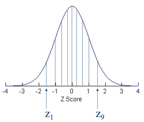
Figure 2
For the one-sample test, we first compute 2n + 1 normal scores, where n is our sample size. This will give us n positive normal scores, and it is these positive scores that we use as our replacement values. Here is some code to calculate normal scores for our small set of fertilizer differences.
i <- 1:(2*6 + 1)
n.scores <- qnorm(i/(2*6 + 2))
n.scores
#>  [1] -1.4652338 -1.0675705 -0.7916386 -0.5659488 -0.3661064 -0.1800124
#>  [7]  0.0000000  0.1800124  0.3661064  0.5659488  0.7916386  1.0675705
#> [13]  1.4652338
Notice that the area between any two of these scores is the same.
pnorm(0.3661064) - pnorm(0.1800124)
#> [1] 0.07142858
pnorm(1.0675705) - pnorm(0.7916386)
#> [1] 0.07142857
We have divided the normal distribution into 14 sections, each with the same area.
We only want the positive scores for our replacement scores.
n.scores <- n.scores[8:13]
n.scores
#> [1] 0.1800124 0.3661064 0.5659488 0.7916386 1.0675705 1.4652338
We now order our fertilizer difference scores based on the absolute values of these differences.
Now that we have the order, we can attach the signs to our normal scores.
n.scores <- n.scores*sign(A.minus.B)
n.scores
#> [1]  0.1800124  0.3661064 -0.5659488 -0.7916386 -1.0675705 -1.4652338
Our test statistic is the sum of the positive difference scores.
Let’s look at the distribution.
rand_dist(n.scores)
#>       T
#>  [1,] 0                 0.0156250 0.0156250 1.0000000
#>  [2,] 0.180012369792705 0.0156250 0.0312500 0.9843750
#>  [3,] 0.36610635680057  0.0156250 0.0468750 0.9687500
#>  [4,] 0.546118726593275 0.0156250 0.0625000 0.9531250
#>  [5,] 0.565948821932863 0.0156250 0.0781250 0.9375000
#>  [6,] 0.745961191725568 0.0156250 0.0937500 0.9218750
#>  [7,] 0.791638607743375 0.0156250 0.1093750 0.9062500
#>  [8,] 0.932055178733433 0.0156250 0.1250000 0.8906250
#>  [9,] 0.97165097753608  0.0156250 0.1406250 0.8750000
#> [10,] 1.06757052387814  0.0156250 0.1562500 0.8593750
#> [11,] 1.11206754852614  0.0156250 0.1718750 0.8437500
#> [12,] 1.15774496454394  0.0156250 0.1875000 0.8281250
#> [13,] 1.24758289367085  0.0156250 0.2031250 0.8125000
#> [14,] 1.33775733433665  0.0156250 0.2187500 0.7968750
#> [15,] 1.35758742967624  0.0156250 0.2343750 0.7812500
#> [16,] 1.43367688067871  0.0156250 0.2500000 0.7656250
#> [17,] 1.46523379268552  0.0156250 0.2656250 0.7500000
#> [18,] 1.53759979946894  0.0156250 0.2812500 0.7343750
#> [19,] 1.61368925047142  0.0156250 0.2968750 0.7187500
#> [20,] 1.633519345811    0.0156250 0.3125000 0.7031250
#> [21,] 1.64524616247823  0.0156250 0.3281250 0.6875000
#> [22,] 1.72369378647681  0.0156250 0.3437500 0.6718750
#> [23,] 1.81353171560371  0.0156250 0.3593750 0.6562500
#> [24,] 1.83134014948609  0.0156250 0.3750000 0.6406250
#> [25,] 1.85920913162152  0.0156250 0.3906250 0.6250000
#> [26,] 1.90370615626951  0.0156250 0.4062500 0.6093750
#> [27,] 1.99962570261157  0.0156250 0.4218750 0.5937500
#> [28,] 2.0113525192788   0.0156250 0.4375000 0.5781250
#> [29,] 2.03118261461839  0.0156250 0.4531250 0.5625000
#> [30,] 2.03922150141422  0.0156250 0.4687500 0.5468750
#> [31,] 2.17963807240428  0.0156250 0.4843750 0.5312500
#> [32,] 2.21119498441109  0.0156250 0.5000000 0.5156250
#> [33,] 2.22531548842209  0.0156250 0.5156250 0.5000000
#> [34,] 2.2568724004289   0.0156250 0.5312500 0.4843750
#> [35,] 2.39728897141896  0.0156250 0.5468750 0.4687500
#> [36,] 2.40532785821479  0.0156250 0.5625000 0.4531250
#> [37,] 2.42515795355438  0.0156250 0.5781250 0.4375000
#> [38,] 2.4368847702216   0.0156250 0.5937500 0.4218750
#> [39,] 2.53280431656366  0.0156250 0.6093750 0.4062500
#> [40,] 2.57730134121166  0.0156250 0.6250000 0.3906250
#> [41,] 2.60517032334708  0.0156250 0.6406250 0.3750000
#> [42,] 2.62297875722947  0.0156250 0.6562500 0.3593750
#> [43,] 2.71281668635637  0.0156250 0.6718750 0.3437500
#> [44,] 2.79126431035495  0.0156250 0.6875000 0.3281250
#> [45,] 2.80299112702217  0.0156250 0.7031250 0.3125000
#> [46,] 2.82282122236176  0.0156250 0.7187500 0.2968750
#> [47,] 2.89891067336423  0.0156250 0.7343750 0.2812500
#> [48,] 2.97127668014765  0.0156250 0.7500000 0.2656250
#> [49,] 3.00283359215446  0.0156250 0.7656250 0.2500000
#> [50,] 3.07892304315694  0.0156250 0.7812500 0.2343750
#> [51,] 3.09875313849653  0.0156250 0.7968750 0.2187500
#> [52,] 3.18892757916233  0.0156250 0.8125000 0.2031250
#> [53,] 3.27876550828923  0.0156250 0.8281250 0.1875000
#> [54,] 3.32444292430704  0.0156250 0.8437500 0.1718750
#> [55,] 3.36893994895503  0.0156250 0.8593750 0.1562500
#> [56,] 3.4648594952971   0.0156250 0.8750000 0.1406250
#> [57,] 3.50445529409974  0.0156250 0.8906250 0.1250000
#> [58,] 3.6448718650898   0.0156250 0.9062500 0.1093750
#> [59,] 3.69054928110761  0.0156250 0.9218750 0.0937500
#> [60,] 3.87056165090031  0.0156250 0.9375000 0.0781250
#> [61,] 3.8903917462399   0.0156250 0.9531250 0.0625000
#> [62,] 4.07040411603261  0.0156250 0.9687500 0.0468750
#> [63,] 4.25649810304047  0.0156250 0.9843750 0.0312500
#> [64,] 4.43651047283318  0.0156250 1.0000000 0.0156250
We can calculate the p value.
The nplearn package contains a function for generating normal scores.
Let’s again draw larger random samples. This time I’ll simulate normally distributed difference scores.
# Obtain 60 normally distributed difference scores with a raw effect size of 2 and a standardized effect size of 0.25.

diff.scores <- rnorm(60, mean = 2, sd = 8)

many.n.scores <- norm_scores(diff.scores)
many.n.scores
#>  [1] -0.40085811  0.56250721 -0.49167259  0.74046747  0.94577709
#>  [6]  0.27035748 -1.04703818 -1.12098304 -0.29173166  1.01213103
#> [11]  1.24504624  0.97841553  0.44580556  2.13468333 -0.51499376
#> [16]  1.50959209  0.88334633 -0.68744352  1.20162669  0.42322495
#> [21]  1.39196028  0.79566030 -0.71370464 -0.66164818 -0.14432239
#> [26] -0.58674192 -0.85339080 -1.73938416 -0.46861583  1.57718007
#> [31] -0.33489417 -0.63628579  1.44827204 -0.02054758 -0.31323996
#> [36]  0.37869006 -0.22796670  0.76777150  1.96702501  1.08327016
#> [41] -0.82418215  2.40003638  0.91411630 -0.04110384  0.35670658
#> [46]  0.20692866  0.61132626  1.16036154 -0.18598182 -0.16511628
#> [51]  0.53859848  1.29094915  0.10291203  0.06167748  1.65285363
#> [56]  1.84132620 -0.12359072  0.08227727  1.33974621  0.24910613
Now we are in the same predicament that we were when we had original scores and wanted to do the Fisher-Pitman test with a large sample. We need to turn to a large-sample approximation.
# Here is our observed value of the test statistic.

TS <- sum(many.n.scores[many.n.scores > 0])

# Here is the mean of T under the null hypothesis.

mu.TS <- 0.5*sum(many.n.scores[many.n.scores > 0])

# Here is the standard deviation of T.

sd.TS <- sqrt(0.25*sum(many.n.scores[many.n.scores > 0]^2))

# This is the Z score.

z <- (TS - mu.TS)/sd.TS

# This is the p value for a one-sided test.

pnorm(z, lower.tail = FALSE)
#> [1] 1.813267e-07
Note that the “jumps” are all different sizes, so we can’t incorporate a correction for continuity, though we did take into account the discrete nature of the data.
Under the null hypothesis, the normal scores are normally distributed. This means that we could use the t.test as a large-sample approximation. The difference is that we are assuming continuous, rather than discrete, data.
t.test(diff.scores, alternative = "greater")
#>
#>  One Sample t-test
#>
#> data:  diff.scores
#> t = 3.1986, df = 59, p-value = 0.001111
#> alternative hypothesis: true mean is greater than 0
#> 95 percent confidence interval:
#>  1.239784      Inf
#> sample estimates:
#> mean of x
#>  2.596064
What if we had done this with normal scores? Given that we have a normal distribution, we should obtain approximately the same result.
t.test(many.n.scores, alternative = "greater")
#>
#>  One Sample t-test
#>
#> data:  many.n.scores
#> t = 3.1319, df = 59, p-value = 0.001351
#> alternative hypothesis: true mean is greater than 0
#> 95 percent confidence interval:
#>  0.1708397       Inf
#> sample estimates:
#> mean of x
#> 0.3662716
I am pleased with these last two results, but using the formula for a large-sample approximation with Z scores gives a result that startles me! I obtained this from a reputable textbook, but now I’m questioning whether it is right. I am going to investigate. In the meantime, I suggest that you use the t test for the large-sample approximation.
What if the difference scores had not come from a normal distribution? In the next example, I’m going to draw them from a uniform distribution.
# Obtain 60 uniformly distributed difference scores with a raw effect size of 2 and a standardized effect size of 0.25.

a <- (4-sqrt(768))/2
b <- 4 - a

diff.scores <- runif(60, a, b)

many.n.scores <- norm_scores(diff.scores)
Now let’s look at the results of the t test with original scores. Notice that the distribution is not normal, but it is symmetrical and we have enough scores to exceed the rule of thumb of 30 and the rule of thumb of 50.
t.test(diff.scores)
#>
#>  One Sample t-test
#>
#> data:  diff.scores
#> t = 3.2729, df = 59, p-value = 0.001782
#> alternative hypothesis: true mean is not equal to 0
#> 95 percent confidence interval:
#>  1.104626 4.580250
#> sample estimates:
#> mean of x
#>  2.842438
Let’s now use the normal scores.
t.test(many.n.scores)
#>
#>  One Sample t-test
#>
#> data:  many.n.scores
#> t = 3.4265, df = 59, p-value = 0.001119
#> alternative hypothesis: true mean is not equal to 0
#> 95 percent confidence interval:
#>  0.1644182 0.6260095
#> sample estimates:
#> mean of x
#> 0.3952138
Should I be concerned that these p values are so different? No! We know that using the t test with the original scores should control our Type I error rate because the distribution is symmetrical and we have a large sample size. What we discover, however, is that by using the large-sample approximation to the nonparametric normal scores test, we obtain substantially more power. Take that all you bloggers who nonchalantly say that you get less power with nonparametric statistics! We’ll explore this issue some more in our next section on relative efficiency.